Elastic

Where developers learn, build, and share. Your source for hands-on demos, cheat sheets, explainers and more.

[Elastic @elastic]

Images fill your context window before the question does.

A single 384px page becomes hundreds of visual tokens. Send
all of them to the LLM and there's no room left to reason.

jina-vlm sits an attention-pooling connector between a
SigLIP2-So400M/14-384 encoder and Qwen3-1.7B-Base. The
connector weighs which visual tokens carry signal, then hands
the text model a smaller set.

Two-stage training, multilingual by design.

Pooling costs you fine detail. Small type inside a dense table
is still hard.

Most people blame the LLM for bad answers on mixed documents.
The trade usually happens at the connector.

Read the paper: https://t.co/ByxK99dshK

[Elastic @elastic]

The HNSW vs DiskBBQ call comes down to recall and budget.

HNSW scales logarithmically and it is genuinely fast, but only while the vectors stay resident. Let them spill and latency climbs exponentially. Indexing pays the same tax, because building the graph means searching the graph.

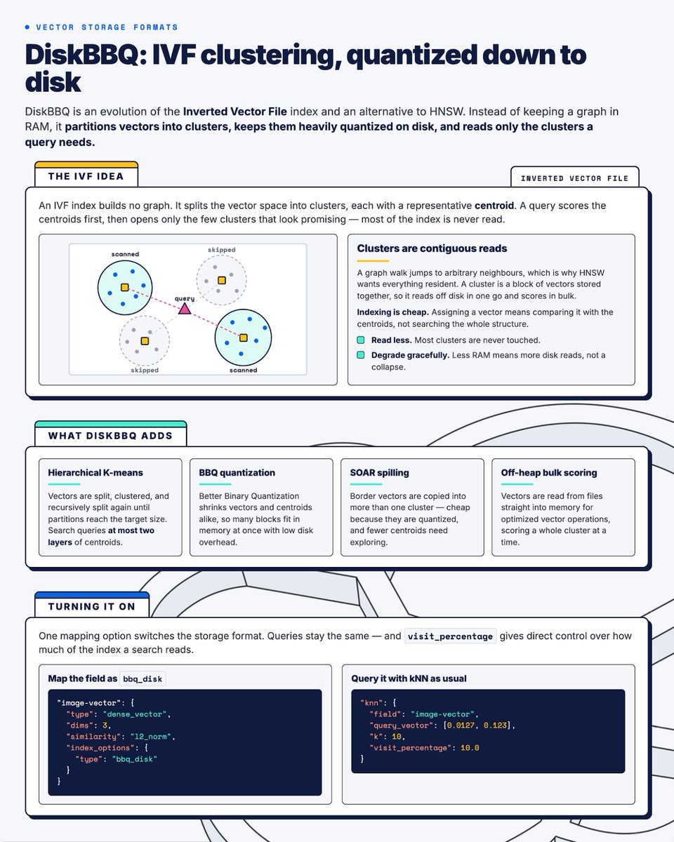
DiskBBQ clusters vectors with hierarchical k-means and keeps them BBQ-quantized on disk, scoring only the clusters a query touches.

Need 99%+ and have the memory budget? Stay on HNSW. Cost-sensitive and fine at 95%?Go with DiskBBQ.

https://t.co/sngyaVXeKm

[Elastic @elastic]

Full design write-up:
https://t.co/s0zIWczev9

[Elastic @elastic]

An AI agent is optimizing Elasticsearch. Engineers validate on improved performance

Coding agents are trained on tasks judged by LLMs and humans. Being convincing gets rewarded. That's a problem when the question is "did this get faster?"

One agent, two phases with different permissions. Exploration goes broad on a real workload and ranks opportunities; a human approves the benchmark and promotes one into a scoped exploitation task. A statistical acceptance rule the agent can't bypass decides whether it lands, and a human reviews before the PR.

All validated with Elasticsearch engineers in the loop

[Elastic @elastic]

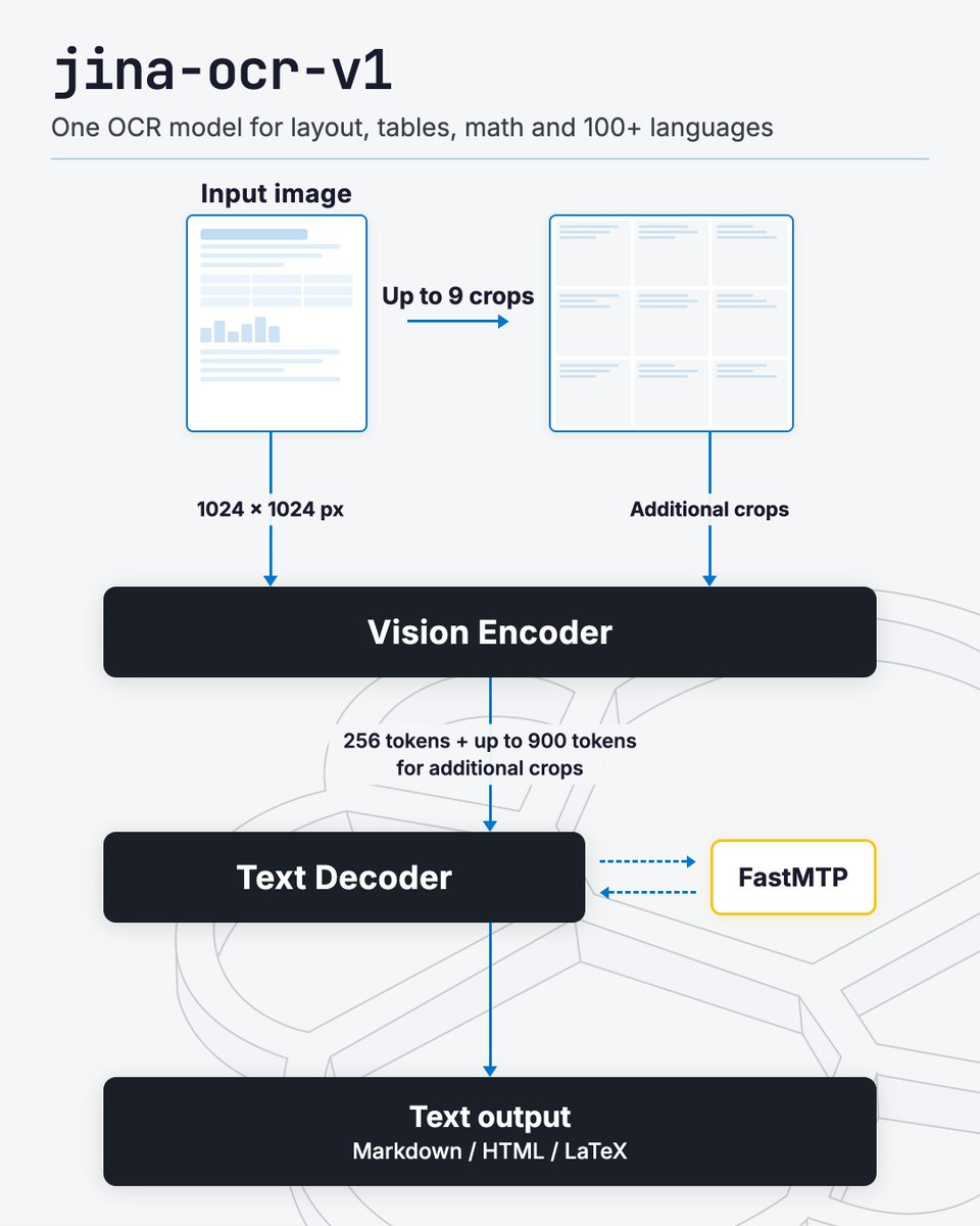
jina-ocr-v1 is now available.

One model covers what otherwise takes a pipeline in OCR: layout, tables, math, handwriting, 100+ languages.

- Scores 83.4 on olmOCR-bench: highest of any OCR model under 600M active parameters
- Scores 91.14 on OmniDocBench, ahead of GPT-5.2 (86.59) and Qwen3-VL-235B (89.78)
- 3.4B total parameters, 570M active: the memory of a 3.4B model, the speed of a 570M one
- Input as PNG
- Output is Markdown, with HTML for tables and LaTeX for math

Also on the Jina API (10M free tokens) with downloadable weights on Hugging Face, CC BY-NC 4.0 licensed for research and noncommercial use.

Blog, technical report, and model card: https://t.co/BYUbRcVBMI

Try it on your own scans via the Jina API, 10M tokens free: https://t.co/HGsTa8DH8F

[Elastic @elastic]

AlertZero: From Alert Noise to Attack Narratives: Relevance Please - Episode 9 https://t.co/vu0v2Vbq6F

[Elastic @elastic]

Full GA details, setup walkthrough, and the per-feature nuances (alerting, SLOs, Synthetics, Streams): https://t.co/wDgO758Cie

[Elastic @elastic]

Cross-project search is GA on Elastic Cloud Serverless.

Search across serverless projects in different regions and cloud providers without moving data.

You can now link up to 100 projects by default (higher limits on request) from project settings in the Elastic Cloud console. Queries hit every linked project automatically. Route your search with project routing by region, cloud, alias, or custom tags. Data access control is consistent and complete wherever you’re querying from using Elastic Cloud API keys.

Works with Security, Observability, Search, and Vector Database project types, including serverless projects you are already running. Complete tier is required for Security and Observability projects.

Link the projects, open Discover, and run a cross-project query today.

[Elastic @elastic]

6,000,000,000 downloads.

If you've ever built on it, deployed it, broken it, fixed it, or shipped something with it: this one's yours.

Thank you.

[Elastic @elastic]

DiskBBQ introduction: https://t.co/wcpvtrz4z8

[Elastic @elastic]

HNSW buys fast search by keeping every vector in RAM.

It needs them there to index too, because indexing means querying the graph you're still building.

DiskBBQ takes the other route:

- Hierarchical k-means groups similar vectors into small clusters
- BBQ compresses each vector 32x
- A query scores nearest centroids, then bulk scores only those clusters

On 1M vectors in memory: 94s to index against 1,054s. Recall 91% against 92%.

That's a point of recall for an order of magnitude on indexing. Above 99% recall the trade stops paying, and HNSW is still the answer.

[Elastic @elastic]

You and your AI agent shouldn't be using curl.

A skill that shells out to curl has a hostname, an API key and a runtime baked in. Change one and it breaks. Worse, the key is in the skill file, so it's in the transcript too.

The Elastic CLI gives every Elasticsearch, Kibana and Cloud API the same shape. Learn elastic es search and you already know how elastic kb data-views list behaves. Agent Skills now run on it.

- API keys stay in your OS keychain, not in flags
- Any command prints its JSON Schema with --help --json
- --dry-run validates input and sends nothing
- commands.allowed in your config decides what an agent can run
- --output-fields cuts a response down to what fits the context window

Tech preview, on npm now: npm install -g (at)elastic/cli

Full write-up, including allowlist config and how universal skills bind HTTP calls to CLI commands: https://t.co/kmhbr2Dgwg

[Elastic @elastic]

Read more: https://t.co/A2fyBF9HBU

[Elastic @elastic]

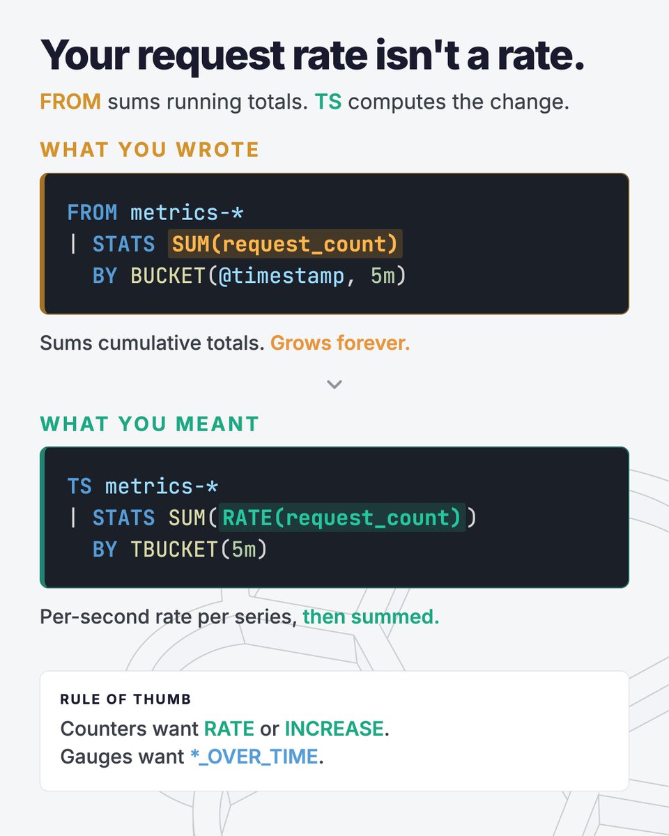
SUM(request_count) in a FROM query is not your request rate.

request_count is a cumulative counter: each sample is the running total since the process started. FROM treats every document as an independent row, so SUM adds each host's running total once per sample. The result isn't a rate, isn't the number of requests in the bucket, and keeps growing even after traffic stops.

FROM metrics-* | STATS SUM(request_count) BY BUCKET(@ timestamp, 5m)

TS is the source command built for this:

TS metrics-* | STATS SUM(RATE(request_count)) BY TBUCKET(5m)

TS groups samples by time series before anything else runs. RATE computes the per-second change inside each series and handles counter resets. SUM then adds those rates across hosts.

That's the shape of every TS query: an inner function per time series (RATE, AVG_OVER_TIME, MAX_OVER_TIME), then a normal aggregate across them (SUM, AVG, MAX). Skip the inner one and TS defaults to LAST_OVER_TIME, which is why TS | STATS AVG(cpu_usage) and FROM | STATS AVG(cpu_usage) return different numbers.

When to use which:
- TS for metric aggregations on a time series data stream. Dashboards, alerts, charts.
- FROM for events: logs, traces, audit records. Each row is independent.
- FROM on a TSDS still works and is useful for inspecting raw metric documents, but it has no per-series semantics.

Pick the inner function deliberately. The outer one is the easy part.

[Elastic @elastic]

Elasticsearch 9.5's columnar index mode stops indexing most fields by default.

So what keeps a range query fast without an inverted index or BKD tree?

2 changes underneath made it possible. Tech preview, read before you switch. https://t.co/5rmUg54p4B

[Elastic @elastic]

OTel Lookup Processor: Relevance Please - Episode 8 https://t.co/nBmY5zzU4N

[Elastic @elastic]

The hard parts of hybrid retrieval, already done.

Elasticsearch Vector Database is a new serverless offering where expert-level tuning is the default:

- bfloat16 storage: half the disk footprint before quantization even starts
- BBQ: up to 32x vector compression, 95% less memory
- Auto-calibration re-tunes quantization on every merge as your data drifts
- Filtered vector search at up to 8x higher throughput than OpenSearch
- Jina AI embeddings and reranking on managed GPU inference, or bring your own models

You bring documents and queries. We handle the embeddings, tuning, and infrastructure.

Full breakdown, including the semantic_text quickstart and what ships in vectorDB index mode: https://t.co/SeeKSeL2aY

[Elastic @elastic]

BM25 has been the default similarity on every Elasticsearch text field since version 5.0. Every lexical query
you have ever run was scored with it (unless you defined otherwise).

That default still does work, vectors can't. Exact tokens are the clearest case: SKUs, error codes, version
numbers, people's names. A dense retriever puts you in the right neighborhood. BM25 lands on the token.

So run both. RRF fuses the two result sets by rank, blending the scores between the two approaches.

[Elastic @elastic]

Blog: https://t.co/PsunfKPnip

Both optimisations ship in Elasticsearch 9.5+ and Elastic Cloud Serverless. Columnar mode is available as a technical preview.

[Elastic @elastic]

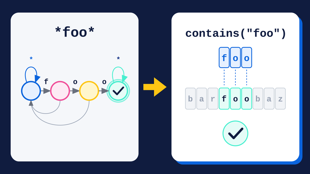
Wildcard queries like *pizza* are 2.3x faster on columnar keyword fields in Elasticsearch 9.5.

The old path builds an automaton for every *term* query and runs state transitions per document. Expensive when you're scanning millions of rows with no inverted index.

The rewrite rule spots the *term* pattern at runtime and swaps in a SIMD substring search instead. Simpler code, wider registers, same result.

A second rule handles empty string filters. SearchPhrase != '' used to decompress Zstd chunks just to check for zero-length values. Now it reads string lengths straight from the offset array: 1.6x faster, skips the Zstd step entirely.

Both rules came from the same habit: run a real query, find the special case, swap in something cheaper.