Carlos Pérez-González

[Mathematica @mathemetica]

Integration by parts turns products of functions into simpler integrals.

If u(x) and v(x) are continuously differentiable, then ∫u dv = uv − ∫v du.
Use the ILATE rule to pick u: Inverse, Logarithmic, Algebraic, Trigonometric, Exponential.

Example: ∫(log x)⋅1 dx = x log x − x + C.

Engineers rely on it to compute work from variable forces in physics and to solve signals in electrical and mechanical systems.

[tetsuo @tetsuoai]

How CNNs see images.

Tensors, filters, feature maps, stride, padding, channels, pooling, receptive fields, mental model.

[Maria Lipiz @matessindramas]

Series de Fourier

[Maria Lipiz @matessindramas]

Así funciona el algoritmo de Dijkstra

[Juan Matías Sepulcre @JMSepulcre]

#LaTeX es una poderosa herramienta para poder escribir #matemáticas de forma impecable. Este manual (2ª ed.) está especialmente dirigido al alumnado, profesorado o investigadores que deseen iniciarse y adquirir soltura en su manejo https://t.co/CUWhQxwQUQ
@PublicacionesUA

[Bastián Olea 🌸 @bastimapache]

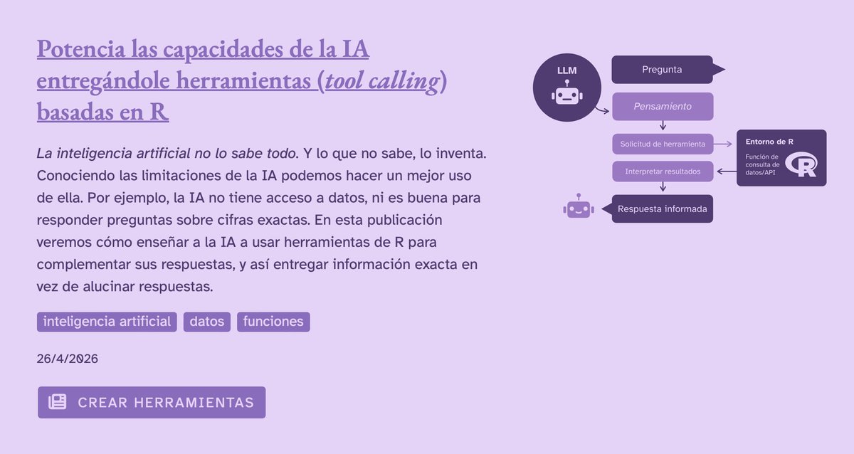
He estado explorando la integración de IA con el lenguaje de análisis de datos R 📊⚙️
Producto de eso he subido varios tutoriales para incluir IA en procesamiento de datos, hacer que la IA acceda a datos con R, crear chatbots especializados, y más! 🤖
👉🏼 https://t.co/62tDG12LCs

[kynd.info @kyndinfo]

Principal Component Analysis 主成分分析
[Math short write-up]
https://t.co/CKulZU34GM

[Bastián Olea 🌸 @bastimapache]

Con R es muy fácil crear sistemas de IA que respondan informados por documentos, estudios y textos! No más respuestas ambiguas ni "alucinaciones" gracias al RAG ⚙️📝
Tutorial: https://t.co/pYFPqesCu6

[Rosana Ferrero 📈📊🙌 @RosanaFerrero]

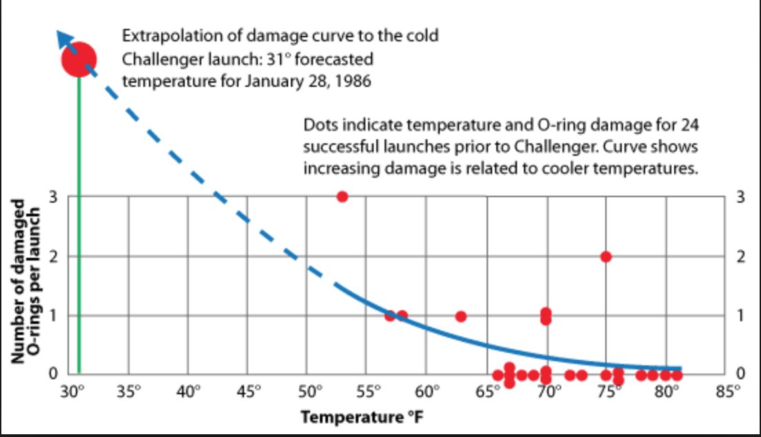
📊El error gráfico que costó 7 vidas y una lección sobre el "Sesgo de Selección"
¿Sabías que el desastre del transbordador espacial Challenger en 1986 no ocurrió por falta de datos, sino por un error catastrófico al elegir cuáles datos mostrar?
Lecciones para tu próximo gráfico👇

[Code Geek @codek_tv]

Same problem, different legends. Which method is your favorite?

[Alex Zajac (🍔,🧠) @itsalexzajac]

An engineer built an interactive book on data structures and algorithms of 680 pages:

[𝗿𝗮𝗺𝗮𝗸𝗿𝘂𝘀𝗵𝗻𝗮— 𝗲/𝗮𝗰𝗰 @techwith_ram]

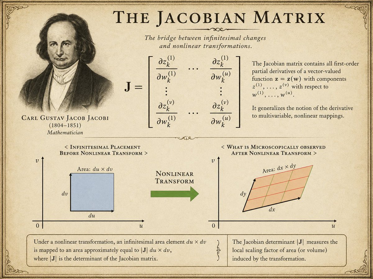
What if I told you a neural network understands local change before it understands the full picture?

That idea is deeply connected to something called the Jacobian Matrix.

At first, it looks terrifying. A big matrix full of partial derivatives. But the intuition behind it is actually beautiful.

The Jacobian measures how small changes in input variables affect the output of a system.

Imagine slightly changing the pixels of an image.
Or changing one feature in a dataset.

How much does the prediction change?
The Jacobian tells us exactly that.

You can think of it as a “sensitivity map” for transformations.

If a system transforms one space into another, the Jacobian describes how the geometry changes locally.

Tiny squares can stretch, rotate, compress, or skew into completely different shapes.

That is why Jacobians are everywhere in AI & machine learning.

For example:

- Backpropagation relies heavily on Jacobians through the chain rule
- Neural networks use them to understand gradient flow
- Normalizing Flows use Jacobian determinants for probability density transformations
- Computer Vision uses them in geometric warping and image alignment
- Robotics uses Jacobians for motion and control systems
- Diffusion models and generative models often depend on transformations between latent spaces

The interesting part is this:
Most ML models are basically learning transformations.

And the Jacobian is what tells us how those transformations behave locally.

Step-by-step intuition:
- Start with an input vector
- Apply a transformation
- Measure how each output changes with respect to each input
- Store those local relationships inside a matrix That matrix becomes the Jacobian.

Carl Gustav Jacob Jacobi introduced this mathematical idea long before AI existed.

But today, modern deep learning silently runs on top of concepts like this every second.

Sometimes the most important parts of AI are not the flashy models.

They are the mathematical structures underneath them.

[数学 for 大学受験 @Mathworld4]

【ガブリエルのラッパ】
𝑦 = 1/𝑥 のグラフをぐるっと回転させてできる図形
🔹 体積 ＝ π（有限）
🔹 表面積 ＝ ∞ （無限）
という面白い結果が得られる。

つまり「中にペンキを満たすことはできるのに、外側を塗り潰すことはできない」ということ。

[Data Science Fact @DataSciFact]

'The most important aspect of a statistical analysis is not what you do with the data, it's what data you use.' -- Andrew Gelman

[Machine Learning Mastery @TeachTheMachine]

Pretraining a Llama Model on Your Local GPU

https://t.co/o77mLpaPir

[Data Science Fact @DataSciFact]

Why are there squares everywhere in statistics (e.g., normal density, variance, least squares, etc.)?

https://t.co/5O2ATZUMS4

[一只小橘呀 @Ellieorange8]

数学系硕士强烈推荐的数学学习资源：awesome-math

其实真正高质量的数学教材、视频、题库，全被整理在一份 GitHub 清单里

Awesome Math，已获 14k+
它把代数、几何、分析、概率、数论等 30+ 领域
全部拆成体系化入口

📌 视频课 + 电子教材 + 练习工具
📌 甚至 MIT、哈佛学生的课程笔记
📌 持续更新，帮你省掉筛选时间

想用数学碾压所有人，直接收藏这份清单：
https://t.co/At3E4YFNbY

[Alexander Inspira IA @Alex_Inspira]

Sigo sin entender, cómo tan poca gente usa herramientas de IA.

La mayoría solo conoce ChatGPT y Claude❌

Aquí tienes 11 JOYAS OCULTAS que necesitas conocer AHORA.

Guárdalo ahora o te arrepentirás👇

[World of Science @Science_TechTV]

Which method speaks to you the most?

[Math Files @Math_files]

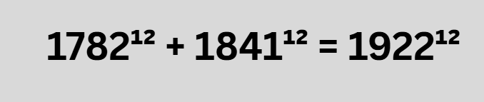
The television show The Simpsons, in the “Treehouse of Horror” episode from the sixth season, revealed the following counterexample to Fermat’s Last Theorem:

1782¹² + 1841¹² = 1922¹²

We leave it as an exercise for you to make peace between this example and Andrew Wiles’s celebrated proof.

Source: Mathematical Apocrypha