Levintsky

@xai. ex-@Google Gemini, ex-@Meta FAIR, ex-@Apple, @Uber, @Baidu, @Adobe. Alumni of @Tsinghua_Uni @UCLA @UofT.

[刘江/LIU Jiang @turingbook]

AI时代就是要敢想啊，太励志了——协和的一个神经外科博士生金山木，本科北大地质专业，自学数学，用GPT-5.6解决了矩阵分析领域一个核心且著名的未解难题Crouzeix猜想（2004年提出）！ 已经得到Crouzeix本人在内的多位数学家确认。 https://t.co/qunH2mq5UE

[Qwen @Alibaba_Qwen]

We promised open weights for Qwen3.8. Now, time to meet them! 🎉

⚡ Qwen3.8-27B:
- A native multimodal dense model. With just 27B parameters, it outperforms Qwen3.7-Plus overall and shines in real-world coding & office workflows.
- 262K native context, easily extendable to 1M tokens via YaRN.
- Built for builders. Highly efficient, high-quality, and licensed under Apache 2.0.

🚀 The open weights for Qwen3.8-2.4T-A95B (Max-level) have also been released recently.

Whether you're shipping lightweight applications with Qwen3.8-27B locally or building agents with Qwen3.8-2.4T-A95B, they're yours now!

Download, deploy, and build something we haven't imagined yet. 👀👇
- Hugging Face：
https://t.co/4kaAcqYEVj
- ModelScope：
https://t.co/eRIMZCGkhC

[Mustafa Suleyman @mustafasuleyman]

Our latest code model is 25% more efficient, higher quality, and a quarter of the cost than our model launched in June. Now live in GitHub Copilot - try it out.

[Artificial Analysis @ArtificialAnlys]

SpaceXAI's Grok 4.6 scores 61 on the Artificial Analysis Intelligence Index, joining the frontier in line with GPT-5.6 Sol, with standout agentic performance at lower cost

Grok 4.6 gains 5 points over Grok 4.5 on the Intelligence Index just over one month after its release, or +23 points compared to Grok 4.3. This brings SpaceXAI back to the intelligence frontier alongside OpenAI, behind only Anthropic.

Key takeaways:
➤ Grok 4.6 joins the frontier of the Artificial Analysis Intelligence Index: It scores 61, in line with GPT-5.6 Sol (max), behind Claude Opus 5 (max, 63) and Claude Fable 5 (max with fallback, 62), and just ahead of Kimi K3

➤ Strong agentic performance: Grok 4.6 achieves a GDPval-AA v2 Elo of 1753, behind only Claude Opus 5 and with overlapping confidence intervals with Claude Fable 5 and Qwen3.8 Max. It scores 50.7% on 𝜏³-Banking, among the top two scores alongside Qwen3.8 Max (51.3%), and 88.4% on Terminal-Bench v2.1, in line with the leading models

➤ Frontier-level intelligence at lower cost: Headline pricing is unchanged from Grok 4.5 at $2/$6 per 1M input/output tokens, 60%+ below Claude Opus 5 ($5/$25) and GPT-5.6 Sol ($5/$30). It cost $0.84 per task, the same as Kimi K3 with slightly higher intelligence, placing it on the Intelligence vs. Cost per Task Pareto frontier

➤ Grok 4.6 sits at Fable 5-tier on AA-Briefcase, our private benchmark of long-horizon agentic knowledge work tasks, with an Elo of 1577 - behind the Claude Opus 5 family. It is notably turn-efficient, completing tasks in ~53 turns and ~0.5B input tokens on average vs. ~103 turns and ~2.0B input tokens for Claude Opus 5 (max)

Other model details:
➤ Context window of 500k tokens (unchanged from Grok 4.5)

➤ Pricing of $2/$6 per 1M tokens of input/output; cache hits discounted to $0.5 per 1M tokens, an increase over Grok 4.5’s $0.3 per 1M tokens for cache hits

Congratulations to @SpaceXAI and @elonmusk on the release!

[Levintsky @Levintsky]

RT @zhu_hanqing666: Now it’s true 🫣

Enjoy Grok 4.6! We built on our previous favorite boy, Grok 4.5 :), refined the recipes with previous…

[Alexander Panfilov @kotekjedi_ml]

We can finally talk about it:

We found a way to extract hidden reasoning of frontier models using a vulnerability in the APIs of every frontier AI company.

We verified that our reasoning token count matches billed API thinking tokens 1:1 for most of the prompts we queried.

[AI at Meta @AIatMeta]

Introducing Muse Glimmer, an open-weight 30B-parameter model optimized for local, always-on agent workflows.

Muse Glimmer delivers strong performance on key agentic use cases and benchmarks compared with leading models in its size category, and is designed to run entirely on consumer hardware like a Mac or PCs with performant GPUs.

In keeping with our long tradition of sharing fundamental AI research, we’re releasing model weights under a permissive Apache 2.0 license.

🧵👇

[Keller Jordan @kellerjordan0]

PSA: Most biglab people now read almost zero papers and understand ICLR/ICML/NeurIPS to be mainly full of overclaims & fraud. (but there are a few diamonds in the rough of course)

[Zhihu Frontier @ZhihuFrontier]

🚀 Alibaba Is Taking Qwen3.8-Max Open-Weight
Alibaba launched Qwen3.8-Max today with 2.4T total parameters, 95B active parameters and a one-million-token context window.
It also says the Max weights and Qwen3.8-27B will be released next week.
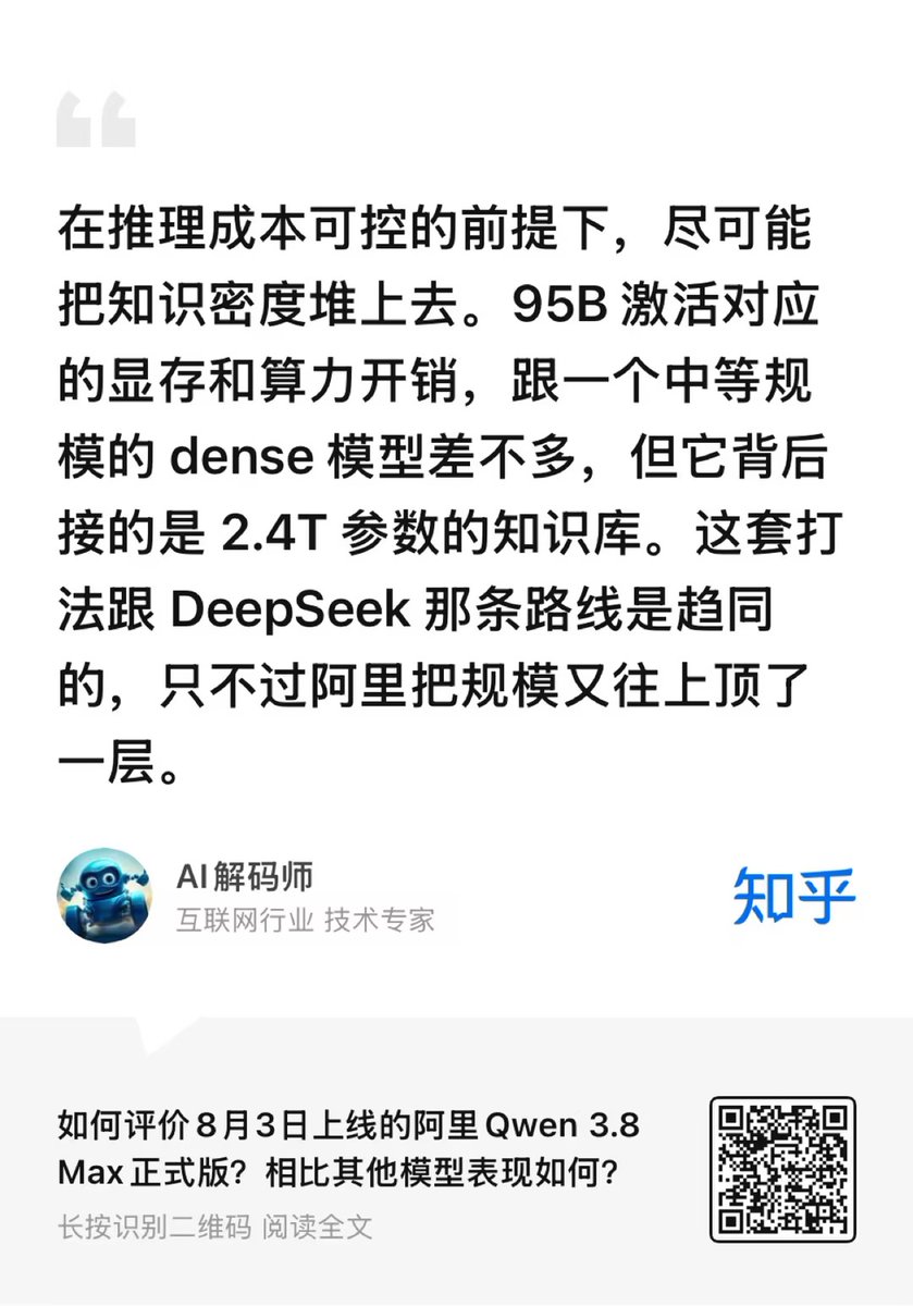
Zhihu contributor AI解码师 sees this as a strategic shift: Alibaba is choosing open ecosystem influence over keeping its strongest model exclusive to paid APIs.

1️⃣ Why open the Max model now?
Alibaba’s previous Max models remained closed, while its open-weight lineup stopped around Qwen3-235B.
The author argues that DeepSeek and other open models have weakened the premium of closed systems. Opening Qwen3.8-Max allows Alibaba to compete for developers, infrastructure support and downstream adoption at the 2.4T scale.

2️⃣ Extreme sparsity keeps inference manageable
Only 95B of Qwen3.8-Max’s 2.4T parameters are activated per token, an activation rate of roughly 4%.
Qwen3-235B-A22B activates close to 10%. Qwen3.8-Max therefore uses much higher sparsity to access a larger parameter pool without paying dense-model inference costs.
The author expects offloading to make experimentation possible for more teams. Actual deployment requirements will remain unclear until the weights, quantized versions and serving tools are released.

3️⃣ Its main strength is long-horizon work
Qwen3.8-Max performs strongly on tasks requiring long contexts and repeated tool use:
🔹 PaperBench: 93.0, ahead of Fable 5 at 88.8
🔹 CoWorkBench: 74.8, close to 75.9
🔹 WideSearch: 81.9, roughly level with 81.2
These benchmarks test paper reproduction, professional work and deep search. The model must preserve one objective across many interactions instead of solving an isolated question.
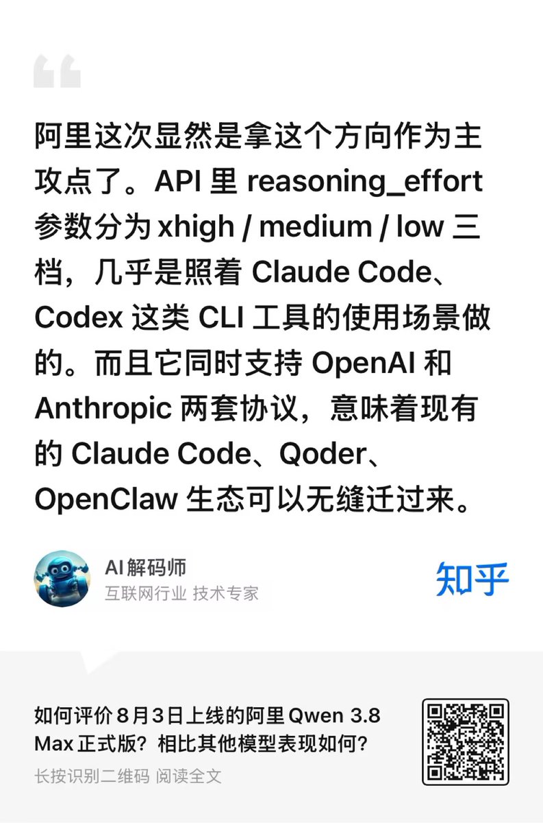
The API also offers low, medium and xhigh reasoning-effort modes. Support for both OpenAI and Anthropic protocols makes it easier to test inside existing coding-Agent workflows.

4️⃣ Real projects show both progress and limits
The author tested Qwen3.8-Max on two coding tasks.
It migrated a Vue 2 component to Vue 3 with performance close to Claude.
On a harder task involving OpenTelemetry instrumentation across a Python service, it missed several edge-case spans. Cross-file reasoning and exhaustive coverage still lag behind the strongest closed models.

5️⃣ The pricing is aggressive
International API pricing is listed at:
· $2 per million input tokens
· $6 per million output tokens
· $0.25 per million cached tokens
According to the author, this is around one-quarter to one-sixth of leading Claude or GPT prices.
Cached input is particularly useful for Agents, which repeatedly reuse long prompts, codebases and tool histories.

🔑 Alibaba’s two-front strategy
Qwen3.8-Max targets closed models with a low-cost API while using open weights to attract researchers, infrastructure providers and private-deployment users.
As frontier models become more accessible, competition will increasingly move toward training data, Agent Harnesses, verification and production infrastructure.

Official release:
https://t.co/aYDH9vUQHw

🔗 Full Reading:
https://t.co/Od5M2bJvyL

#Qwen38Max #Alibaba #OpenModels #AIAgents #CodingAgents #AIInfrastructure

[Benhao Huang @huskydogewoof]

🔥
𝐍𝐞𝐰 𝐛𝐥𝐨𝐠: 𝐓𝐨𝐰𝐚𝐫𝐝𝐬 𝐋𝐨𝐨𝐩𝐞𝐝 𝐌𝐨𝐝𝐞𝐥𝐬 𝐃𝐨𝐧𝐞 𝐑𝐢𝐠𝐡𝐭 — 𝐏𝐚𝐫𝐭 𝐈

Looped models reuse the same weights across depth, promising a better compute–parameter trade-off, especially for reasoning.

𝐁𝐮𝐭 𝟏) 𝐝𝐨 𝐭𝐡𝐞 𝐠𝐚𝐢𝐧𝐬 𝐬𝐮𝐫𝐯𝐢𝐯𝐞 𝐰𝐡𝐞𝐧 𝐛𝐨𝐭𝐡 𝐭𝐫𝐚𝐢𝐧𝐢𝐧𝐠 𝐚𝐧𝐝 𝐢𝐧𝐟𝐞𝐫𝐞𝐧𝐜𝐞 𝐅𝐋𝐎𝐏𝐬 𝐚𝐫𝐞 𝐦𝐚𝐭𝐜𝐡𝐞𝐝? 𝟐) 𝐀𝐧𝐝 𝐰𝐡��𝐜𝐡 𝐚𝐫𝐜𝐡𝐢𝐭𝐞𝐜𝐭𝐮𝐫𝐚𝐥 𝐜𝐡𝐨𝐢𝐜𝐞𝐬 𝐚𝐜𝐭𝐮𝐚𝐥𝐥𝐲 𝐦𝐚𝐭𝐭𝐞𝐫?

We run 𝐚𝐩𝐩𝐥𝐞𝐬-𝐭𝐨-𝐚𝐩𝐩𝐥𝐞𝐬 ablations spanning Ouro to Huginn. Huginn performs better overall, with the largest gains coming from the loop-in-the-middle (sandwich) design and input injection, though they provide different benefits.

Trained on 𝟓𝟎𝟎𝐁 tokens, an 𝟖𝐁-𝐀𝟎.𝟖𝐁 Huginn MoE approaches or surpasses a 𝟑𝟐𝐁-𝐀𝟑.𝟐𝐁 feedforward MoE on several reasoning benchmarks, including GSM8K (83.6% vs. 80.8%), while using 𝟕𝟓% 𝐟𝐞𝐰𝐞𝐫 resident parameters under 𝐦𝐚𝐭𝐜𝐡𝐞𝐝 𝐭𝐫𝐚𝐢𝐧𝐢𝐧𝐠 𝐚𝐧𝐝 𝐢𝐧𝐟𝐞𝐫𝐞𝐧𝐜𝐞 FLOPs.

More details and the blog link in the thread ↓

[Chong Wei 韦冲 @weichonginsight]

最近邓煜获得菲尔兹奖后接受专访，主持人是同为菲尔兹奖获得者陶哲轩的女儿。

在交谈中，他介绍了和合作者用严格数学证明，搭起了从牛顿粒子力学、 玻尔兹曼方程、 流体方程的完整推导链条，攻克了困扰数学界125年的希尔伯特第六问题。

被问及AI，他分享了一个细节：自己花5天证出的引理，GPT一小时内给出了更短的证明。

他说："我们不是在与AI竞争，而是与AI合作去实现以前做不到的事。"

[jianlin.su @Jianlin_S]

Deconstructing Scaling Laws: The Triad of Optimization, Architecture, and Data
https://t.co/jbqiFXsIJN

[Zhihu Frontier @ZhihuFrontier]

Kimi K3 Scales Across Length, Depth, and Width

@Kimi_Moonshot AI has released Kimi K3’s full model weights, technical report, and three pieces of training infrastructure: MoonEP, FlashKDA, and AgentEnv.
The release reveals how K3 scales a 2.8T-parameter MoE model to a 1M-token context window while activating only 104B parameters per token.
Zhihu contributor kaiyuan breaks the architecture down along three axes: sequence length, network depth, and model width.
Moonshot reports that the combined architecture and data improvements deliver roughly 2.5x higher scaling efficiency than Kimi K2.

1️⃣ Sequence: KDA handles length efficiently
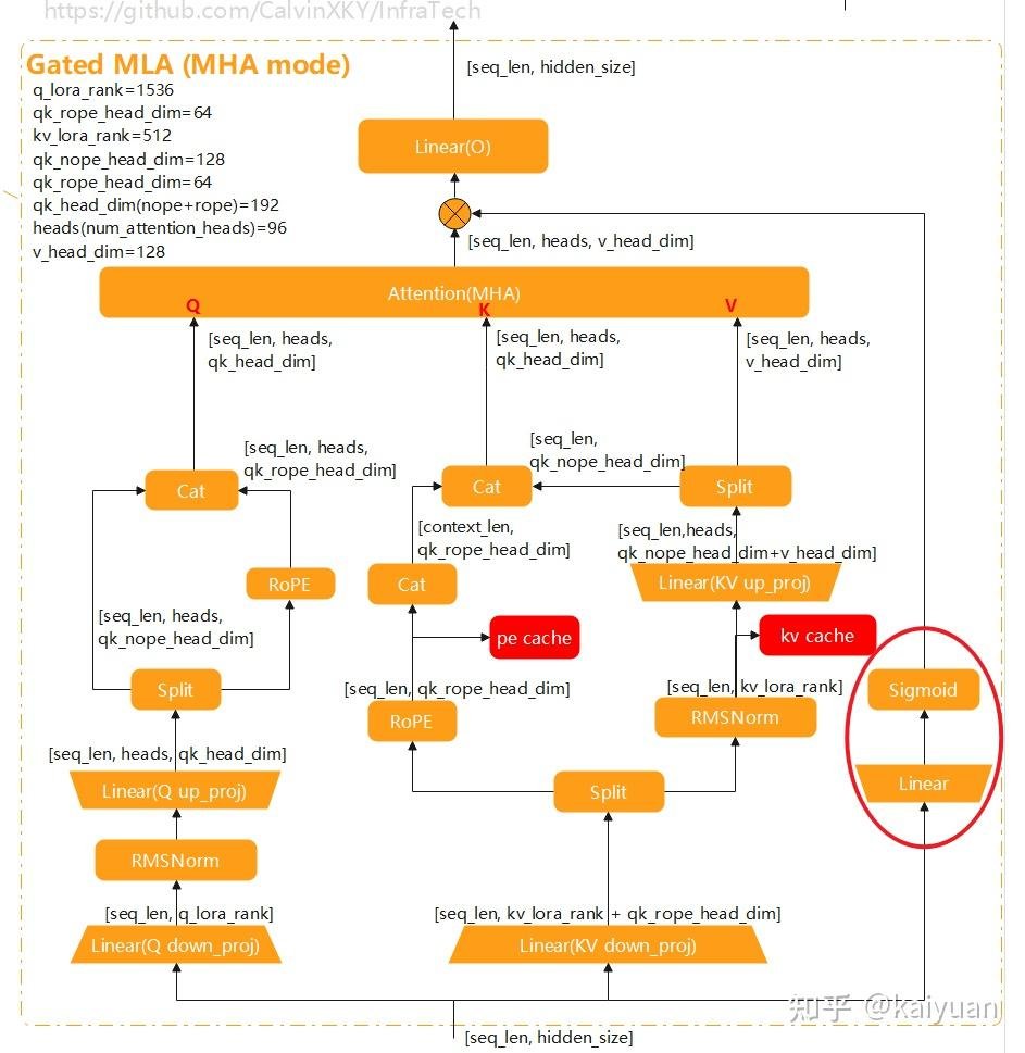
K3 contains 69 KDA layers and 24 Gated MLA layers, following an approximate 3:1 ratio.
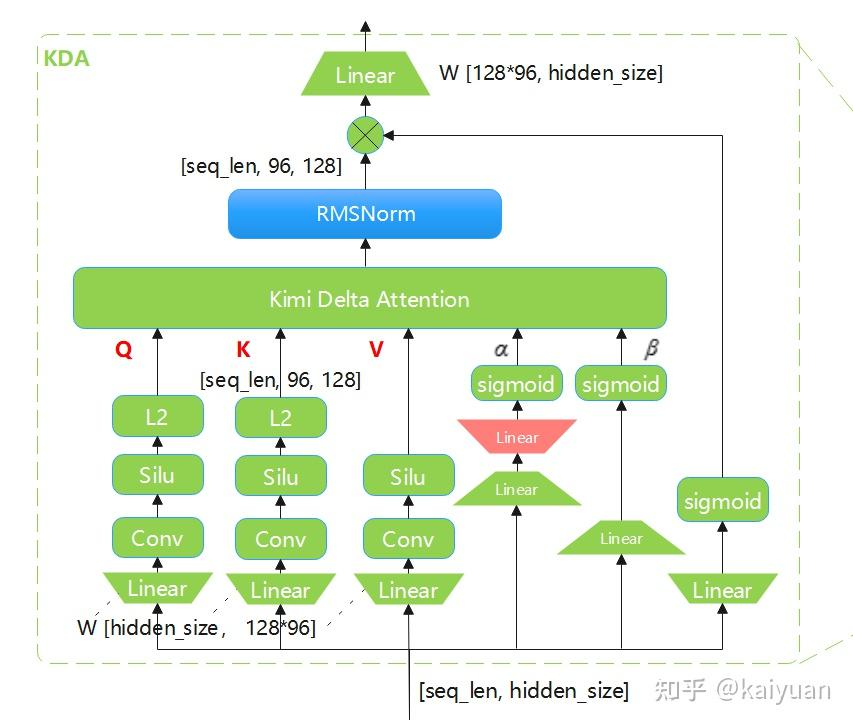
🔷 Kimi Delta Attention
Standard attention stores a growing KV cache. KDA instead compresses history into a fixed-size recurrent state, making long-context processing more efficient.
Its key change over Gated DeltaNet is the decay mechanism.
Gated DeltaNet applies one scalar decay rate to the entire state. KDA predicts multiple decay values, allowing different state dimensions to forget information at different speeds.
🔸 Why retain Gated MLA?
Linear attention is efficient, but its fixed-size state limits how much history it can preserve.
K3 therefore keeps 24 Gated MLA layers for global token interaction. These layers use 96 attention heads and add a sigmoid output gate before the final projection.
The result is a hybrid design: KDA carries most of the long-context workload, while Gated MLA periodically restores full global interaction.

2️⃣ Depth: AttnRes retrieves earlier representations
Standard Transformer residuals add every previous layer with fixed weight.
As models grow deeper, early features can become diluted and hidden-state magnitude can become harder to control.
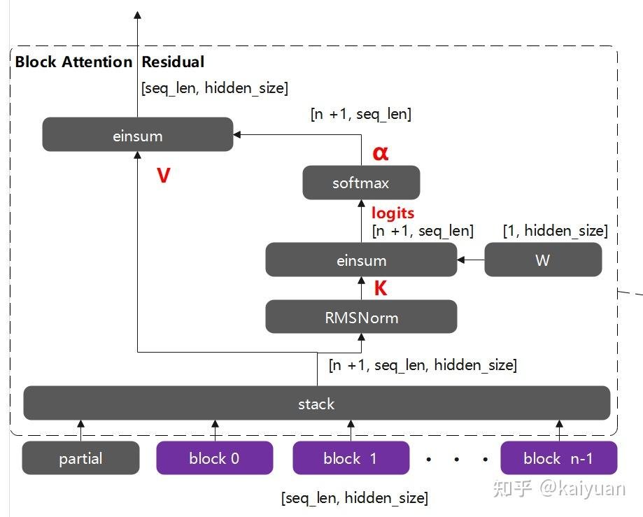
Attention Residuals, or AttnRes, turns the residual pathway itself into attention.
Instead of treating all previous representations equally, each layer learns which earlier features are most useful for the current input.
🔷 Block AttnRes
Full AttnRes would require access to every previous layer, creating high memory overhead.
K3 divides its 93 layers into blocks. Residual accumulation remains conventional inside each block, while attention-based retrieval operates across block boundaries.
This preserves most of the benefit while keeping the additional cost practical.
Information in K3 therefore moves in two directions: across tokens through KDA and MLA, and across depth through selective residual retrieval.

3️⃣ Width: Stable LatentMoE expands capacity
K3 pushes sparsity much further than its predecessors.
Each token selects 16 routed experts from a pool of 896, alongside two shared experts.
This creates enormous total capacity without activating the full 2.8T parameters for every token.
The challenge is keeping such a sparse system stable.
🔷 Quantile Balancing
Expert allocation is derived from router-score quantiles. This reduces dependence on sensitive heuristic load-balancing updates.
🔸 SiTU-GLU
K3 replaces SwiGLU with a bounded activation design. This helps control extreme activations when routing becomes highly sparse.
🔷 Training stability
Per-head Muon provides finer optimization for individual attention heads, while balanced expert parallelism reduces throughput fluctuations caused by uneven routing.
K3 also uses quantization-aware training from the SFT stage, with MXFP4 weights and MXFP8 activations.

4️⃣ Vision: MoonViT-V2 brings native multimodality
K3 uses the approximately 401M-parameter MoonViT-V2 vision encoder.
Images and video frames are converted into patches, encoded, merged into fewer visual tokens, and projected into the language model’s hidden space.
Compared with the previous MoonViT, V2 keeps a similar parameter count while changing its width, attention layout, normalization, and multimodal projector.
Its maximum image patch limit also increases from 16,384 to 65,536, allowing higher-resolution visual inputs.

5️⃣ The open release includes the infrastructure layer
Alongside the weights and technical report, Moonshot also released:
🔹 MoonEP: high-performance communication for large expert-parallel MoE training
🔹 FlashKDA: an optimized KDA kernel for faster long-context prefill
🔹 AgentEnv: isolated sandbox infrastructure for large-scale agent training
This matters because K3 is not only a model architecture. Its scale depends on communication, kernels, routing stability, low-precision training, and distributed agent environments working as one system.
👉 The core idea is simple: K3 does not scale through parameter count alone. It redesigns information flow across length, depth, and width, then supports those changes with matching infrastructure.

📄 Technical report:
https://t.co/wX9h27qchr

💻 Official repository:
https://t.co/SrUHcxTpHJ

🤗 Model weights:
https://t.co/h1EgsEmAr5

🔗 Full Reading:
https://t.co/GgTe8Qlomn

#KimiK3 #MoonshotAI #OpenWeights #MixtureOfExperts #AIInfrastructure #LongContext #MultimodalAI

[elie @eliebakouch]

this scaling law is a piece of art, kimi K3 recipe improves by ~2.5x over kimi K2 recipe

the tech report is amazing

[Sebastian Raschka @rasbt]

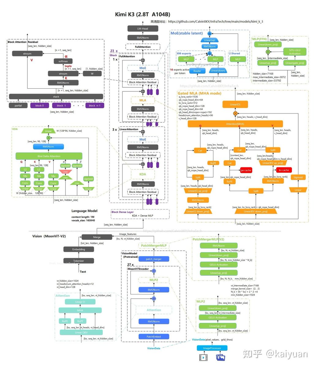
The Kimi K3 architecture figure for yesterday's big open-weight model release, along with some observations and thoughts.

1. Yes, it looks relatively complicated, but it's essentially a scaled-up production version of their Kimi Linear model they released last year (scaled up from 48B -> 2.8T; K3 is by far the biggest open-weight model right now)

2. The one new component compared to Kimi Linear is the LatentMoE. I omitted it in the figure below since it's already very crowded, but that's essentially the same LatentMoE as in Nemotron 3 Ultra (you can find it in my LLM Architecture Gallery if you are curious). The idea here is to compress (down-project) large linear layers similar to multi-head latent attention.

3. Kimi K3's overall trend (similar to Nemotron 3, DeepSeek V4, and others) is also towards better inference efficiency. That is, there are many components that replace existing components with efficiency-tweaked versions. I.e., MoE -> LatentMoE, regular attention -> multi-head latent attention and Kimi Delta Attention. (I also have short tutorials and write-ups in my gallery if you are curious about additional details).

4. The one component change that is not an efficiency tweak is attention residuals. Like DeepSeek V4 improved the residual path with mHC (manifold-constrained Hyper-Connections), attention residuals are a way to improve the residual path, but it works a bit differently. I.e., mHC made the residual path wider. Attention residuals (also already part of Kimi Linear) connect the residuals across layers; the connection itself uses an attention score for an important/contribution weight. According to the report, it improves the validation loss and downstream performance (a bit) consistently and adds about 4% in training cost and 2% in inference cost.

5. Interestingly, Kimi K3 got rid of all RoPE layers and uses NoPE (No Positional Embeddings) everywhere instead. (Again, this is inherited from Kimi Linear). In other architectures, the recent trend was towards RoPE in local attention layers (like sliding window attention) and NoPE in the global layers. There were a few architectures that only used NoPE everywhere, but this is the first frontier-level one as far as I know.

6. Kimi K3 now also has native multimodal support, which is great!

There are several other interesting training tidbits in the technical report, but that's it from the architecture front so far. A really great release overall.

[Susan Zhang @suchenzang]

open-source is beautiful, indeed

[Kimi.ai @Kimi_Moonshot]

Releasing the model weights and technical report of Kimi K3.

Kimi K3 is our most capable model: a 2.8T MoE model with native visual understanding and a 1M-token context window.

New model architecture: 2.5x the intelligence per unit of compute, not just more params.

Alongside Kimi K3, we're opening up more of the stack behind it — high-performance attention kernels, MoE communication library, and infrastructure for running agent environments at scale.

Model weights: https://t.co/7m7eEg6Y0B
Tech report: https://t.co/yeu6cjpMCT
Tech blog: https://t.co/YTfiMSNM1f

[青稞社区 @qingke_ai]

xHC 首次把语言模型的残差流高效扩展到 16 流。

在 18B 和 28B MoE 语言模型的预训练实验中，xHC 在 DeepSeek Manifold-constrained Hyper-Connections (mHC) 的基础上，把收益又提升了近一倍，是目前同 FLOPs 下最强的残差流改进方法之一（包括 Kimi Attention Residual）。 https://t.co/tpi89PDSZH

[Muyu He @HeMuyu0327]

I found it to be lesser known that the standard definitions of KL estimator in RL losses produce the wrong gradients for expected KL.

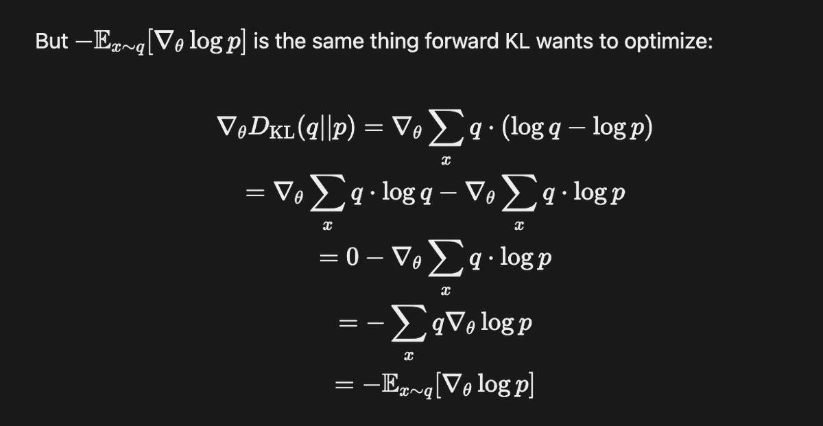
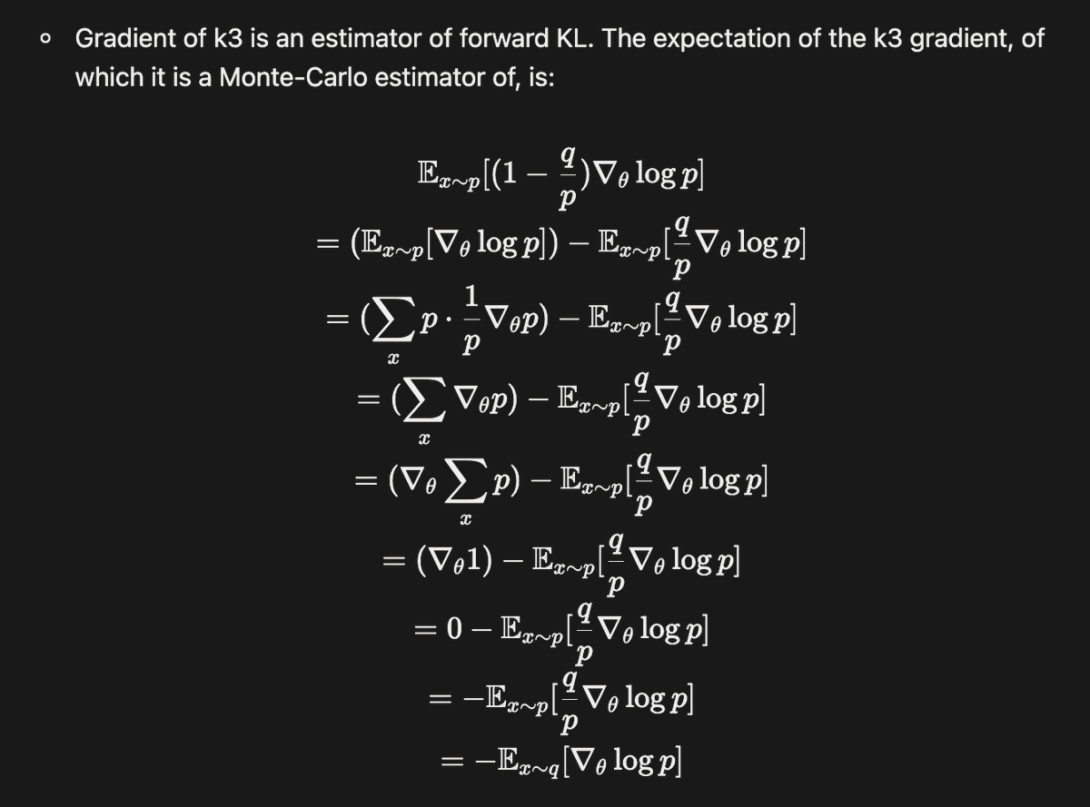
For example, I stumbled upon the discovery that while the k3 estimator (used in DeepSeek series) is an unbiased estimate for the value of expected reverse KL, its gradient is incorrect for the gradient of KL. It's worse: the gradient is actually an unbiased estimate for the gradient of expected forward KL. So k3 estimator as is defined does the opposite of what it tries to do (p1-2).

Then I went deeper into this rabbit hole, after my colleague recommended this paper: https://t.co/6nf3NEG7od. I find two addition things adopted by verl and prob some tech reports that don't make sense:

- that the original k1 estimator, which is just the raw log ratio, produces a gradient of an expectation of 0: essentially it is trying to optimizing nothing (p3).

- that the sequence-level KL, while its value is correctly the sum of all token-level KL, does not have its gradient as the sum of all token-level KL gradients (p4).

I had a great time reading this fascinating paper because it shows how the correct token and sequence KL losses should be defined to yield the right expected gradients. I put my full derivation in a blog because I had fun working out every step: https://t.co/H0bmdHALYc

The coolest thing when deriving the gradient-correct sequence-KL estimator is: although the loss term (and the gradient) as is written is computationally heavily, there are one mathematical trick and one computational trick to make the complexity much lower. One is to find an unbiased, lower-variance formulation; the other is to compute the key sum-of-log-ratio term with .cumsum so the whole thing becomes easy.

I also find that there is an optional path in verl which does something that kinda of makes sense: there is a 'k3+' estimator that does forward in k3 and backward in k2 (0.5 * log_ratio^2). k2 is biased as an estimator of token-KL value but its gradient checks out to be unbiased as an estimator of token-KL gradient. So this is a way to get the right gradient with backward and the right monitoring signal with forward, using the k2 - k2.detach() + k3.detach() trick.