In the last posts, we focused on Curve’s market design and how StableSwap changed the way liquidity can be traded.
But there is another problem that had to be solved before @CurveFinance could scale,
How do you govern a system that controls billions of dollars in liquidity incentives without turning it into a short-term speculation game?
At first glance, governance in DeFi seemed straightforward.
You issue a token.
You give holders voting rights.
You let the market decide.
But this model introduced a structural issue that became visible very quickly across early DeFi protocols.
Voting power was tied almost entirely to ownership, not commitment.
That meant someone could acquire a large amount of governance tokens, influence a decision, and then exit their position immediately after.
The system rewarded capital presence, not long-term alignment.
Curve approached this differently.
Instead of asking “Who owns the most CRV?”, it asked a more fundamental question,
“Who is actually aligned with the long-term success of the protocol?”
This shift led to one of the most important governance designs in DeFi, vote escrow (ve) aka: venomics.
The idea behind vote escrow is simple, but its implications are not.
Instead of using CRV directly for governance, users lock their tokens for a fixed period of time.
In return, they receive veCRV, a non-transferable representation of voting power.
The key detail is that veCRV is not just a 1:1 wrapper of locked tokens.
It is a function of two variables.
The amount of CRV locked and the duration of the lock
The maximum lock period is 4 years.
If someone locks CRV for the full 4 years, they receive maximum voting power.
If they lock for a shorter period, their voting power scales down proportionally.
Over time, this voting power decreases as the remaining lock duration shrinks.
This is what is referred to as "linear decay".
It means voting power decreases gradually as the remaining lock time gets closer to zero..
This design creates a very specific incentive structure.
Short-term participants receive limited governance influence.
Long-term participants are rewarded with disproportionately higher control.
In other words, influence is no longer just purchased, it is earned through time.
But veCRV is not only a governance mechanism.
It also plays a direct role in how liquidity incentives are distributed across Curve.
Holders of veCRV can vote on gauges, which determine where CRV emissions are allocated.
On top of that, veCRV holders receive additional benefits, including:
A share of trading fees generated by Curve pools and boosted rewards for providing liquidity, with boosts reaching up to 2.5x depending on veCRV balance relative to liquidity position
This creates a feedback loop,
Liquidity providers are incentivized to acquire veCRV.
veCRV holders influence where liquidity incentives go.
And those incentives determine where liquidity flows.
What emerges is a full incentive engine for liquidity distribution.
Another critical design choice is that veCRV is non-transferable.
It cannot be traded, sold, or moved between wallets.
This prevents governance power from becoming a purely speculative asset that can be quickly bought and dumped.
Instead, influence is always tied to locked commitment over time.
Looking at this system as a whole, veCRV did not simply modify governance.
It fundamentally changed its structure.
It shifted DeFi governance from a model based on capital ownership to a model based on time-weighted commitment.
And that idea became the foundation for everything that followed, from curve wars, to bribe markets and the federation of protocols building around curve.
Next, we will look deeper at how this voting power is actually used in practice through Curve’s gauge system, and why it turned liquidity allocation into one of the most competitive mechanisms in DeFi.
ngl this bear market has me questioning: is now the time to build or the time to wait? feels like every OG says "build" but my wallet says otherwise 💀
Build X first 👀
In the previous post, I pointed to the bigger idea behind @CurveFinance, stable assets should not be forced into a pricing model that was built for volatile pairs.
That is exactly where StableSwap starts to matter.
If you look at the first graphic, the basic logic is actually quite intuitive.
Alice deposits equal value into the pool, in this case USDT and USDC and receives LP tokens in return.
Those LP tokens are not just a receipt.
They represent her share of the pool.
So when she enters, she owns a proportional claim on the assets inside the pool, and when she exits, she gets her share back based on what the pool looks like at that moment.
That is important, because the pool itself is not static.
The second graphic shows what happens once the pool is no longer perfectly balanced. After a large swap, the reserve composition changes.
One side gets heavier, the other side gets lighter.
In the example, the pool ends up more tilted toward USDC, and that shift is exactly what creates the small profit shown on the withdrawal side.
Alice is not being paid a special reward.
She is simply withdrawing her share of a pool that now holds a different mix of assets than when she entered.
That is also why the example shows the system recovering from imbalance over time.
A StableSwap pool is built so that trades around the peg are very cheap, which is why the curve is so flat near equilibrium.
In the example , a large USDC swap pushes the pool away from balance and moves the price slightly upward, to around 1.002 USDC per $crvUSD.
At that point the pool is no longer perfectly symmetric, and that imbalance itself creates an arbitrage opportunity.
Traders are now incentivized to bring the pool back toward equilibrium by swapping in the underrepresented asset and taking out the other one at a slightly better rate.
That is how the pool naturally moves back toward balance.
So the “positive slippage” or better execution on one side is not a contradiction.
It is part of the mechanism.
Curve concentrates liquidity very tightly around the peg, which means the pool can absorb large trades efficiently near 1.00.
But once the pool is pushed off balance, the pricing function starts reacting more strongly, and that reaction is what keeps the system from staying stuck in an unhealthy state.
This is where the StableSwap design really differs from a simple constant product AMM.
It is about shaping the pool so that liquidity is deepest where stable assets actually trade, while still allowing the system to correct itself when one side gets too dominant.
This behavior is governed by the StableSwap invariant and the amplification coefficient A, which controls how flat the curve stays around the balanced point.
The higher the amplification, the more liquidity is concentrated near the peg, and the smaller the slippage for trades that happen close to equilibrium.
So if I had to put the whole example into one sentence, I’d say this:
Curve builds a pricing system that rewards balance, reacts to imbalance, and uses arbitrage to push the pool back toward the state it was designed for.
In the previous post, we established why constant product AMMs fail to efficiently handle stable assets, and why @CurveFinance had to rethink the entire pricing problem from first principles.
Now we can finally look at what Curve actually built instead.
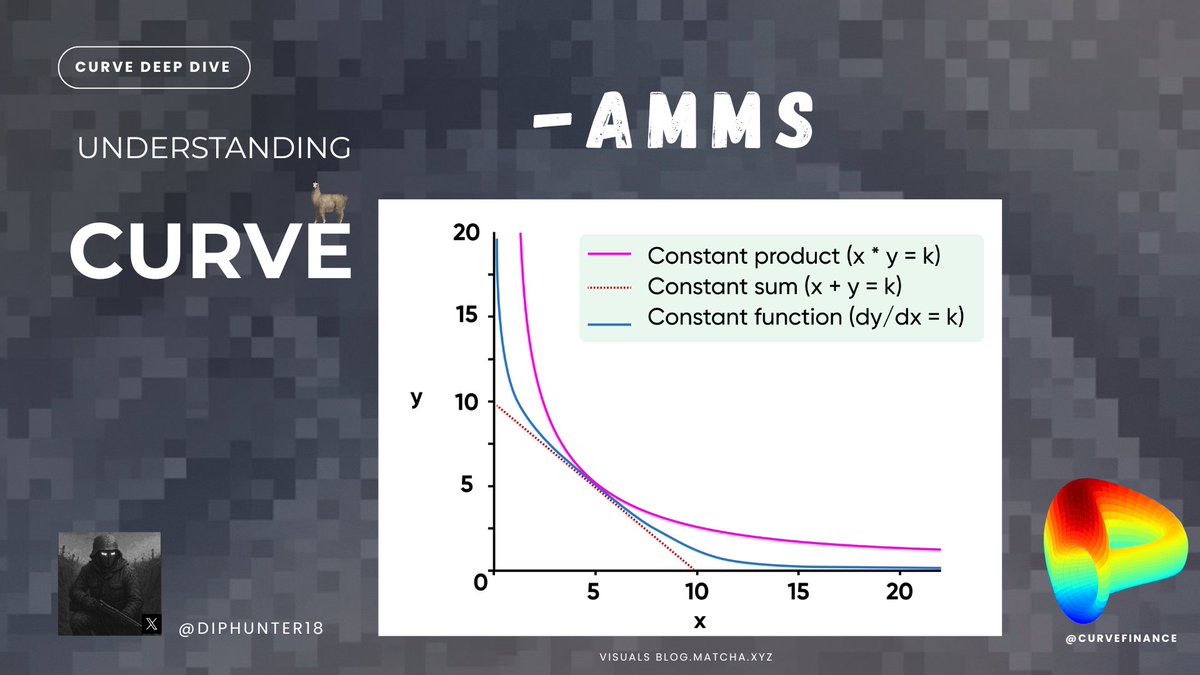
The StableSwap Invariant is a hybrid system that blends two fundamentally different market behaviors into a single continuous curve.
To understand why this matters, it helps to revisit the two extremes we discussed earlier.
On one end, there is the constant product market maker.
It assumes that price should always respond to imbalance. As one asset is removed from the pool, the remaining reserves become increasingly expensive. This ensures liquidity is always preserved, but at the cost of higher slippage.
On the other end, there is the constant sum model.
Here, trades occur almost perfectly at a fixed ratio. There is virtually no slippage near equilibrium. But this comes at a critical cost: liquidity can be completely drained from one side of the pool without meaningful price adjustment.
Neither system is sufficient on its own.
Constant product is too conservative for stable assets.
Constant sum is too fragile.
One additional implication of this design becomes visible when looking at impermanent loss.
In constant product AMMs, impermanent loss is a structural consequence of price divergence between assets. As prices move away from the initial deposit ratio, LPs are effectively rebalanced into the underperforming asset, which creates value loss relative to simply holding.
StableSwap reduces this effect significantly under normal market conditions because liquidity remains concentrated around the equilibrium price range. Since most trading activity happens near the 1:1 region, rebalancing effects are minimized as long as the peg holds.
However, this does not eliminate impermanent loss entirely. In extreme depeg scenarios, the system can still behave like a constant product AMM as imbalance grows, meaning LPs remain exposed to downside risk when one asset loses its peg.
Curve’s insight was that stable asset markets do not live at the extremes.
They spend most of their time clustered around a known equilibrium price, but occasionally experience stress events where deviation becomes significant.
This observation is what the StableSwap design is built around.
Instead of forcing the entire curve to behave like one model, Curve introduces a dynamic structure that changes depending on how balanced the pool is.
Near equilibrium, the pricing function behaves almost like a constant sum system.
This means extremely low slippage even for large trades, because the system assumes that both assets should trade at nearly identical value.
But as the pool becomes increasingly imbalanced, the curve gradually shifts its behavior.
Price impact begins to increase more aggressively, eventually resembling the protective characteristics of a constant product AMM.
This transition is continuous, which is the key design choice behind StableSwap.
The system effectively adapts its “conservatism” based on risk.
When assets are balanced, it prioritizes efficiency.
When imbalance grows, it prioritizes liquidity protection.
To control how sharp or flat this transition behaves, Curve introduces a parameter known as the amplification coefficient (A).
Intuitively, A determines how strongly the system “believes” that the assets should stay at parity.
A higher A value means the curve stays flatter for longer around the equilibrium price, allowing larger trades with minimal slippage.
A lower A value makes the system behave more like a standard constant product AMM, reacting faster to imbalance.
This single parameter is what allows Curve pools to be tuned for different types of correlated assets, from tightly pegged stablecoins to more loosely correlated assets.
What makes this design powerful is not just the reduction in slippage.
I sincerely doubt the number is that high. Insane if so.
But the point about using a low float high FDV token to strike deals for exclusive integrations still stands.
People used to say to me all the time at Euler: “do more BD.”
But lack of integrations almost always was nothing to do with BD efforts. Very few people we didn’t speak to during my time there.
It almost always came down to money. “So and so are offering X millions for an exclusive integration, what can you do?”
I assume most of those types of deals were done with tokens and not real $ because the numbers were often eye watering.
And we had 1/100th of budget or less than competitors because of the depressed EUL token price. So we would always get excluded or pushed aside once someone else came in.
Sometimes people talked to us enthusiastically one day and completely ghost us the next once they’d agreed a deal elsewhere.
With the benefit of hindsight I think we should have tried to take Euler private and start again with the token.
But hindsight is a wonderful thing. It wasn’t the same regulatory environment as we have now and there were lots of arguments against doing that.
The point is that you really need a highly valued token to compete for liquidity and integrations in lending though. The tech is very much secondary to your ability to pay in the early years to bootstrap liquidity and integrations.
It does make me wonder what will happen when all these pay to play token holders start to take profit after vesting ends or hedge out their exposure though.
In the previous post, we looked at why @CurveFinance was created and the problem it set out to solve.
Now let's take a closer look at why existing AMMs couldn't solve that problem in the first place.
Most decentralized exchanges rely on a constant product market maker, commonly represented by the formula x · y = k.
It's one of the most elegant ideas in DeFi.
As one asset leaves the pool, the ratio between the two reserves changes, causing the price to adjust automatically.
No order books.
No centralized market makers.
Just a mathematical invariant that continuously discovers prices through supply and demand.
For assets whose prices naturally fluctuate against each other, like ETH and USDC, that model works remarkably well.
Price discovery is exactly what the market needs.
If demand for ETH increases, the AMM should make ETH more expensive.
If demand falls, the price should decline accordingly.
The invariant continuously reflects those changing market conditions.
Now imagine a completely different market.
USDC against USDT.
Or DAI against USDC.
These assets aren't competing with each other.
They're designed to represent the same underlying value.
Under normal market conditions, the expected equilibrium price isn't unknown.
It's already approximately 1:1.
Yet the AMM doesn't understand that.
It applies exactly the same pricing model it would use for ETH and USDC.
Every swap moves the pool further away from balance.
As the imbalance grows, execution becomes increasingly expensive and slippage rises, even though both assets are still supposed to be worth the same amount.
This wasn't a flaw in the constant product model.
It was simply solving a different problem.
Constant product AMMs are designed to discover prices.
Stable asset markets don't primarily need price discovery.
They need efficient exchange around an already known equilibrium.
That distinction is what changed Curve's entire design philosophy.
Instead of asking how to improve the constant product formula, @newmichwill started by questioning the assumption behind it.
What if the market already knows the fair price?
What if the goal isn't discovering value, but preserving it while allowing massive amounts of liquidity to move with as little friction as possible?
Those questions completely redefine the optimization target.
A pricing function for stable assets shouldn't try to push prices apart after every trade.
It should do the exact opposite.
It should keep prices as close as possible to parity for as long as liquidity remains balanced.
At first glance, you might think the solution would simply be using a constant-sum model (x + y = k).
A constant-sum curve would allow assets to trade almost perfectly at 1:1 with virtually no slippage.
But that creates an even bigger problem.
cause the price barely changes, traders could completely drain one side of the pool while continuing to trade at nearly the same price.
Eventually, one asset would disappear entirely.
The pool would stop functioning.
In other words, constant product protects liquidity but sacrifices efficiency.
Constant sum maximizes efficiency but sacrifices liquidity.
Neither model solves both problems at once.
Curve's breakthrough wasn't choosing one over the other.
It was combining the strengths of both.
Near equilibrium, StableSwap behaves much more like a constant-sum market, allowing extremely large trades with minimal slippage.
As the pool becomes increasingly imbalanced, the curve gradually transitions toward constant-product behavior, preventing liquidity from being completely drained.
The result is a market that remains highly efficient when assets stay close to their intended value, while still retaining the self-correcting properties that make AMMs resilient under stress.
This hybrid approach became the StableSwap Invariant.
Over the next couple of days/weeks, I'm going to give you a deep dive into @CurveFinance.
By building an understanding from the ground up.
My goal is simple, by the end of this series, you should understand not only what Curve is, but why it became one of the most important pieces of infrastructure in DeFi.
The more I learned about Curve, the more I realized that it was built to solve a very specific problem and that's exactly why it became so successful.
Imagine you hold a million USDC and want to swap it for USDT.
On a traditional automated market maker, a trade of that size would move the price significantly.
The larger the trade, the more value you lose to slippage.
Curve asked a simple question,
What if both assets are supposed to have almost the same value in the first place?
If USDC and USDT are both designed to trade around one dollar, why should swapping between them become increasingly expensive as trade size grows?
That question became the foundation of Curve.
Instead of optimizing for every possible trading pair, Curve was specifically designed for assets that are expected to trade at similar prices stablecoins, liquid staking tokens, wrapped assets, and other closely correlated assets.
That single design decision completely changed the economics of on-chain trading.
It allowed users to execute significantly larger swaps with far lower slippage than traditional AMMs could offer under the same conditions.
Over time, this made Curve the preferred liquidity venue for many of DeFi's largest stablecoin markets.
Today, countless protocols either source liquidity from Curve directly or build products around it.
In many cases, users don't even realize they're interacting with Curve's liquidity because another protocol sits between them and the underlying pools.
This first post is only the starting point.
In the next part, we'll look at why traditional AMMs struggle with stable assets in the first place and why Curve had to invent an entirely different approach instead of simply improving the existing one.