Damian Flores

[Damian Flores @22df_araujo]

De las últimas fotos de mi papá…gracias por tanto maestro 🙏

[Damian Flores @22df_araujo]

Maleza y hierba muy crecida entre el tramo de la empresa AUMA y la Colonia Valle de San Lorenzo, enfrente de la UAAAN, propicia fauna nociva, inseguridad para transeúntes y poca visibilidad para conductores que salen de la colonia @CICsal @SaltilloGob @policiasaltillo

[Josep Ferrer @iamjosepferrer]

Logistic Regression clearly explained 👇🏻

[Matt Dancho (Business Science) @mdancho84]

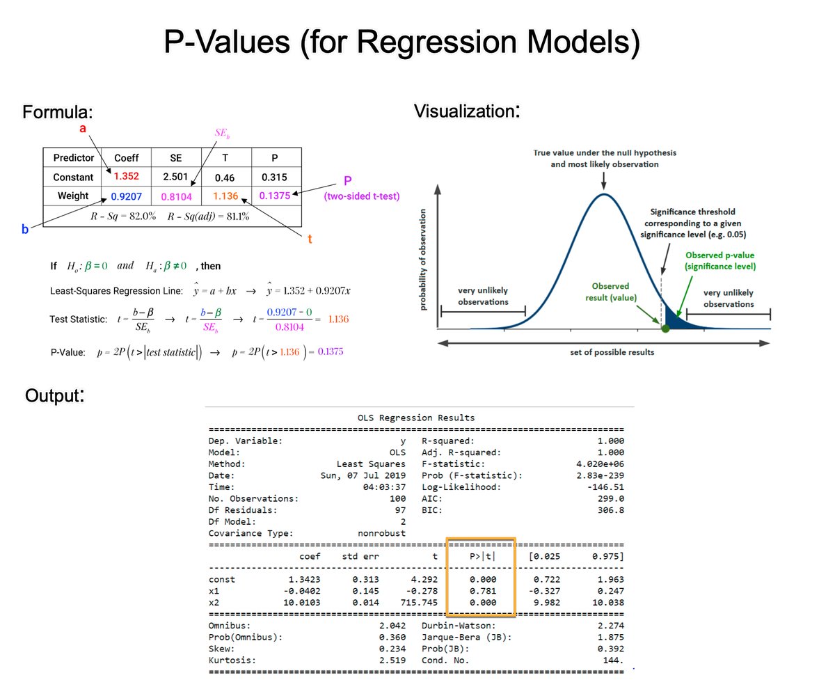
Understanding P-Values is essential for improving regression models. In 2 minutes, learn what took me 2 years to figure out.

1. The p-value: A p-value, in statistics, is a measure used to assess the strength of the evidence against a null hypothesis.

2. Null Hypothesis (H0): This is a general statement or default position that there is no relationship between two measured phenomena or no association among groups. For example, the regressor does not affect the outcome.

3. Alternative Hypothesis (H1): This is what you want to test for. It is often the opposite of the null hypothesis. For example, that the regressor does affect the outcome.

4. Calculating the p-value: The p-value for each coefficient is typically calculated using the t-test. There are several steps involved. Let's break them down.

5. Coefficient Estimate: In a regression model, you have estimates of coefficients (β) for each predictor. These coefficients represent the change in the dependent variable for a one-unit change in the predictor, holding all other predictors constant.

6. Standard Error of the Coefficient: The standard error (SE) measures the accuracy with which a sample represents a population. In regression, the SE of a coefficient estimate indicates how much variability there is in the estimate of the coefficient.

7. Test Statistic (T): The test statistic for each coefficient in a regression model is calculated by dividing the Coefficient Estimate / Standard Error of the Coefficient. This gives you a t-value.

8. Degrees of Freedom: The degrees of freedom (df) for this test are usually calculated as the number of observations minus the number of parameters being estimated (including the intercept).

9. P-Value Calculation: The p-value is then determined by comparing the calculated t-value to the t-distribution with the appropriate degrees of freedom. The area under the t-distribution curve, beyond the calculated t-value, gives the p-value.

10. Interpretation: A small p-value (usually ≤ 0.05) indicates that it is unlikely to observe such a data pattern if the null hypothesis were true, suggesting that the predictor is a significant contributor to the model.

There you have it- my top 10 concepts on p-values. The next problem you'll face is how to apply data science to business.

I'd like to help.

I’ve spent 100 hours consolidating my learnings into a free 5-day course, How to Solve Business Problems with Data Science. It comes with:

300+ lines of R and Python code
5 bonus trainings
2 systematic frameworks
1 complete roadmap to avoid mistakes and start solving business problems with data science, TODAY.

👉 Here it is for free: https://t.co/YXG4pL97ZN

[Prof Lennart Nacke, PhD @acagamic]

Excellent tips for writing a literature review

(from Professor Hall)

[Scholarship for PhD @ScholarshipfPhd]

Abstract Structure

#Research #PhD #academictwitter #postdoc #scholarshipfphd

[Scholarship for PhD @ScholarshipfPhd]

How to get your Paper Accepted for Publication (1/3)

[filipe @filicroval]

El 99% de las empresas utiliza Microsoft Excel.

Pero la mayoría de la gente no tiene ni idea de cómo utilizarlo.

Aquí tienes 7 trucos que debes conocer:

[Matt Dancho (Business Science) @mdancho84]

Probability distributions are critical to data science and business decision-making. In 3 minutes, I'll unpack 3 years of mastering probability distributions for business. Let's go.

1. Probability Distribution Basics: In statistics, a probability distribution is a mathematical function that provides the probabilities of occurrence of different possible outcomes in an experiment. It's a way to describe how likely different outcomes will occur. There are two main types of probability distributions: Discrete and Uniform.

2. Discrete: These are used when the set of possible outcomes is discrete (i.e., can be counted). For example, the number of customers that convert in a time period (which can only take on the values 1, 2, 3, 4, 5, 6, etc).

3. Continuous: These are used when the set of possible outcomes can take on any value in a range. For example, the conversion rate of customers in a given time period is N_conv / N_total, which divides customers (discrete) by the total number of website visits. The resulting conversion rate is continuous.

4. Probability Functions (PDF and PMF): This is how we calculate the probability of an event occurring. Discrete probabilities have a Probability Mass Function (PMF). Continuous probabilities have a Probability Density Function (PMF).

5. Expected Value (IMPORTANT, THIS IS WHAT I USE TO MAKE DECISIONS!): Arguably the most important concept in my opinion is the concept of Expected Value (EV). The expected value is like the long-run average or most typical outcome. I use this to make business decisions. Here's an example.

6. Lead Scoring Model Example: I made a basic logistic regression model that helped my team know which quotes to work on. The model predicted a class probability from 0 to 1, 0 being not likely to buy and 1 being 100% likely to buy. From this we can calculate the Expected Value. Probability of buy x Value of Purchase.

There you have it- my top 6 concepts on probability. The next problem you'll face is how to apply data science to business.

I'd like to help.

I’ve spent 100 hours consolidating my learnings into a free 5-day course, How to Solve Business Problems with Data Science. It comes with:

300+ lines of R and Python code
5 bonus trainings
2 systematic frameworks
1 complete roadmap to avoid mistakes and start solving business problems with data science, TODAY.

👉 Here it is for free: https://t.co/YXG4pL97ZN

[CIC Saltillo @CICsal]

*VÍA DAÑADA* Reportan pavimento dañado con una serie de baches en calz Antonio Narro entre la empresa AUMA y la entrada a la universidad (UAAAN) #Saltillo 09:10 @OPublicasSalt @SaltilloGob https://t.co/BgVLOIHYzF

[Damian Flores @22df_araujo]

@cabrowns Pues que puedes esperar de esas gentes clasistas mi estimado, abrazo

[Matt Dancho (Business Science) @mdancho84]

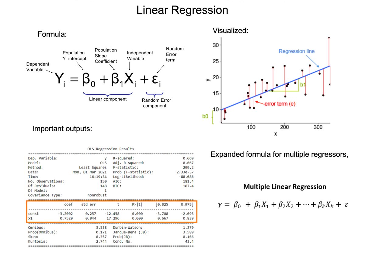
Linear Regression is one of the most important tools in a Data Scientist's toolbox. Here's everything you need to know in 3 minutes.

1. Ordinary Least Squares (OLS) Regression: Aims to find the best-fitting linear equation that describes the relationship between the dependent variable (often denoted as Y) and independent variables (denoted as X1, X2, ..., Xn).

2. OLS does this by minimizing the sum of the squares of the differences between the observed dependent variable values and those predicted by the linear model. These differences are called "residuals."

3. "Best fit" in the context of OLS means that the sum of the squares of the residuals is as small as possible. Mathematically, it's about finding the values of β0, β1, ..., βn that minimize this sum.

4. Slopes (β1, β2, ..., βn): These coefficients represent the change in the dependent variable for a one-unit change in the corresponding independent variable, holding other variables constant.

5. R-squared (R²): This statistic measures the proportion of variance in the dependent variable that is predictable from the independent variables. It ranges from 0 to 1, with higher values indicating a better fit of the model to the data.

6. t-Statistics and p-Values: For each coefficient, the t-statistic and its associated p-value test the null hypothesis that the coefficient is equal to zero (no effect). A small p-value (< 0.05) suggests that you can reject the null hypothesis.

7. Confidence Intervals: These intervals provide a range of plausible values for each coefficient (usually at the 95% confidence level).

Understanding and interpreting these outputs is crucial for assessing the quality of the model, understanding the relationships between variables, and making predictions or conclusions based on the model.

====

Want help improving your data science skills?

Free 10 Skills Webinar: I put together a free on-demand workshop that covers the 10 skills that helped me make the transition to Data Scientist: https://t.co/LR39RJ5XKB

10X Faster Projects w/ ChatGPT: I have a live workshop where I'll share how to use ChatGPT for Data Science (so you can complete projects 10X faster): https://t.co/EaMpKrJiqX

If you like this post, please reshare ♻️ it so others can get value.

[Abacus.AI @abacusai]

Calculus made easy

This is an excellent resource to learn calculus.

And it's free!

https://t.co/5pEfgObr96

[Selçuk Korkmaz @selcukorkmaz]

🧵 Understanding Heteroscedasticity: A Medical Guide

1/ 🤔 What's Heteroscedasticity?
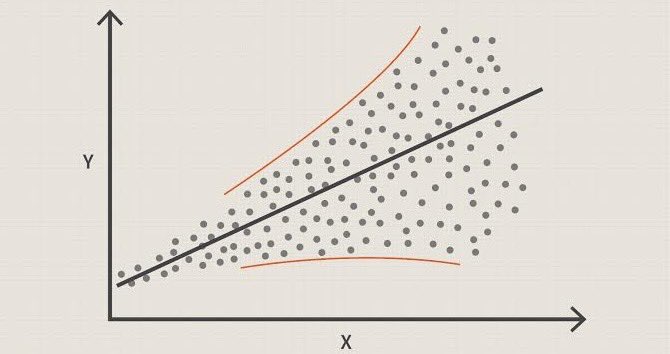
Imagine you're trying to predict a patient's blood pressure based on their age. If the spread of blood pressure readings varies widely at different ages, that's heteroscedasticity. In simple terms, it's when the spread or scatter of your data isn't consistent.

2/ 📈 Why Should We Care?
In medicine, accurate predictions are crucial. When heteroscedasticity is present, it can make our estimates unreliable. This can lead to incorrect conclusions or diagnoses.

3/ 🎯 Consistent vs. Inconsistent Spread
Think of measuring blood pressure in patients. If, at a certain age range, readings are pretty consistent, that's "homoscedasticity" (consistent scatter). But if, as patients age, some have extremely high readings while others remain normal, that's heteroscedasticity (inconsistent scatter).

4/ 🌡️ Real-world Example
Consider age vs. bone density. Young adults might have consistently strong bones. But as people age, some might have severe bone density loss (osteoporosis) while others don't. This varying spread of bone density can be a sign of heteroscedasticity.

5/ 🛠️ How to Spot It?
Plot your data! If you see a funnel shape (narrow at one end, wide at the other), that's a classic sign. There are also formal tests like the Breusch-Pagan or White's test to detect it.

6/ 💡 What Causes It?
Many things! In our bone density example, perhaps factors like diet, exercise, or genetics play a role in the varying spread of results as people age.

7/ 🌟 Fixing Heteroscedasticity
There are several ways:
• Transformations: Like taking the log of your data.
• Adding Variables: Maybe there's a missing piece in the puzzle. In the bone density case, adding calcium intake could help.
• Weighted Regression: Giving different weights to different data points.

8/ 📚 In Conclusion
Heteroscedasticity might sound complex, but in medicine, spotting it ensures our diagnoses and treatments are accurate. Recognizing and addressing heteroscedasticity helps us provide better care! 🌡️

#Statistics #DataScience

[Giuseppe Cavaliere @CavaliereGiu]

Hi #EconTwitter!

Need to wrap up some slides on introductory econometrics? Or looking for theory and practical exercises, including datasets?

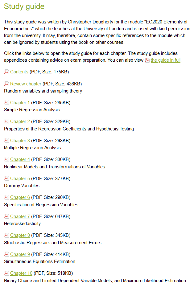
Check out the material associated with Christopher Dougherty's intro #econometrics book. Lots of interesting stuff, including a "study guide" with over 300 pp. of exercises.

Very useful! ⭐️

Links

Resource page: https://t.co/1B8bpV2kU5

Study guide (PDF): https://t.co/MyZc1FF1Yv

[𝖪𝖾𝗇𝗂𝖺 𝗅𝗈 𝗁𝖺𝖼𝖾 𝗍𝗈𝖽𝗈 𝗆𝖺𝗅 @RelatocuriosoK]

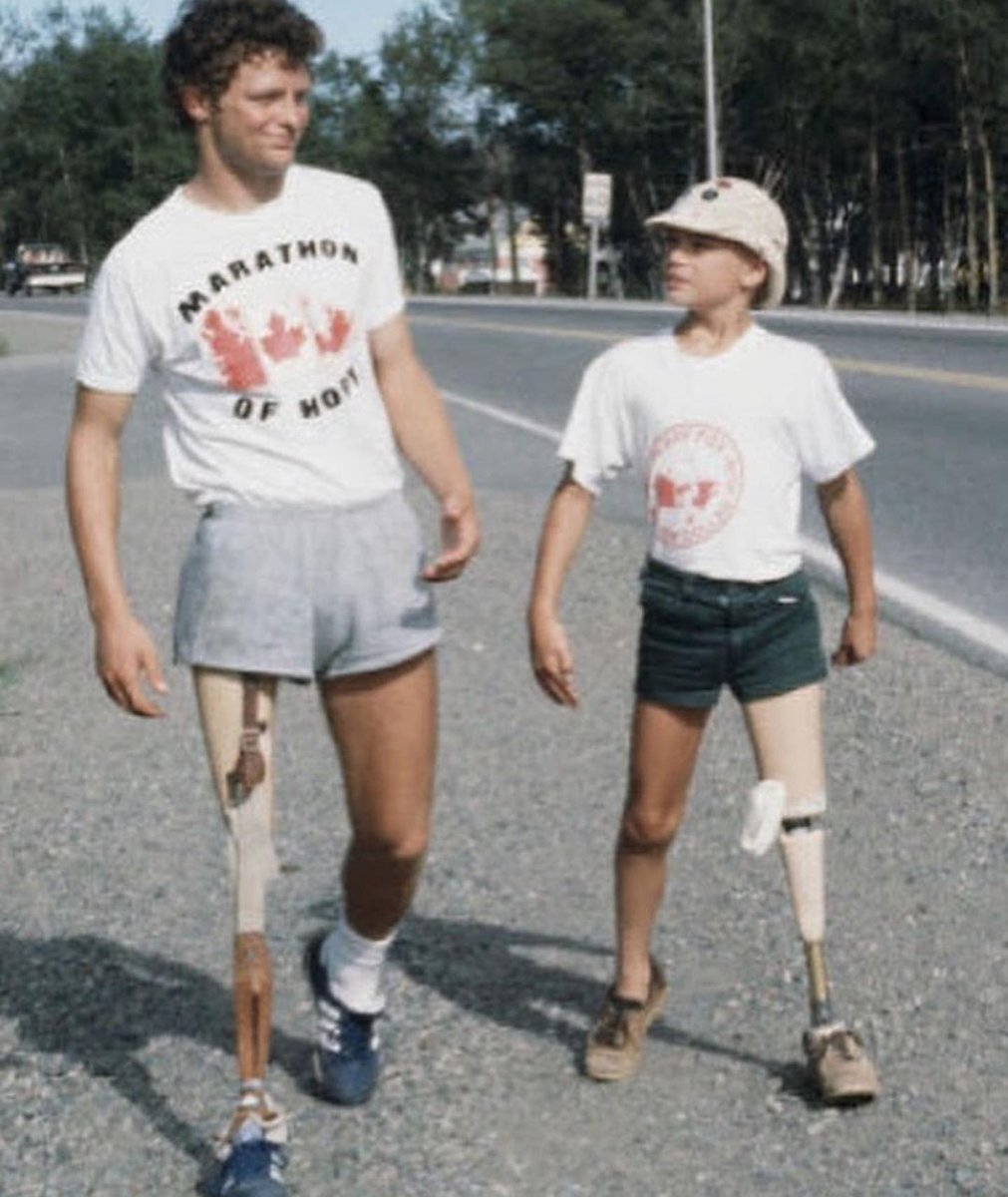
Terry Fox nació en 1958 en Canadá y cuando apenas había cumplido 18 años le diagnosticaron un osteosarcoma: un tipo de cáncer de huesos que le hizo perder la pierna derecha (se trata de un cáncer que suele comenzar atacando la rodilla y que puede propagarse de forma rápida por todo el cuerpo).

Fox, que había sido jugador de baloncesto en el instituto, siguió jugando en silla de ruedas (y llegó a ganar tres campeonatos nacionales) y, ayudado con una pierna ortopédica, comenzó a correr con el fin de recaudar fondos para la investigación del cáncer. Y corrió un maratón diario durante más de cuatro meses.

Instauró lo que él mismo llamó Maratón de la Esperanza, recorriendo Canadá para crear conciencia sobre el cáncer y recaudar fondos para la investigación de la enfermedad. Quería llegar desde Terranova, con costa al Océano Atlántico, hasta Victoria, que da con el Pacífico, donde al final de su aventura habría recorrido unos 8000 kilómetros. Sin embargo, tuvo que detenerse en Thunder Bay, Ontario, cuatro meses y más de 5000 kilómetros después de haber iniciado su proyecto, ya que el cáncer había invadido sus pulmones.

Menos de un mes después Terry Fox murió, pero su legado sigue vivo aun en nuestros días: desde 1981 la "carrera Terry Fox" se celebra anualmente en más de 60 países y está considerada como la mayor carrera de un día destinada a la recaudación de fondos para la investigación del cáncer en todo el mundo.

[Major League Soccer @MLS]

LIONEL ANDRÉS MESSI IS NOT HUMAN.

[Oxfam México @oxfammexico]

¿Existe un modelo económico que beneficie a las personas en situaciones de marginación?
Sí, se llama economía social y aquí te explicamos su importancia 👇
Abrimos 🧵

[Analistas APP descárgala @SomosAnalistas_]

Su papá puede comprar toda Sudamérica si quiere y todavía le pregunta que si puede meter el cereal

Tqm Ciro 🥹🥹

[GEOPOL 21 @Geopol21]

📆Un día como hoy, pero en 1944, tiene lugar el Desembarco de Normandía.

📍Conocida con el nombre en clave de Overlord, los desembarcos aliados en #Normandía marcarían el comienzo de una larga y costosa campaña para liberar el noroeste de #Europa de la ocupación alemana.

[Daniel Ibarra Andrade @d_ibarra]

Argentina: *Agota las entradas al concierto de Taylor Swift en 30 segundos

El FMI: