Kunal Bhashkar

#AILead #AI #ML #DL #RL #AILead #risk #taker #pursuing #PhD #JNU #TechM #Pune
Deep reinforcement learning (DRL) enthusiastic

[Kunal Bhashkar @BhashkarKunal]

#CPT #SLM #GenAI #EWC #Catastrophic #Forgetting
https://t.co/8ubfVHX5Hv

[Kunal Bhashkar @BhashkarKunal]

𝐖𝐡𝐞𝐧 𝐬𝐨𝐜𝐢𝐞𝐭𝐲 𝐠𝐢𝐯𝐞𝐬 𝐟𝐚𝐦𝐞, 𝐬𝐮𝐜𝐜𝐞𝐬𝐬, 𝐚𝐧𝐝 𝐰𝐞𝐚𝐥𝐭𝐡, 𝐠𝐢𝐯𝐢𝐧𝐠 𝐬𝐨𝐦𝐞𝐭𝐡𝐢𝐧𝐠 𝐩𝐨𝐬𝐢𝐭𝐢𝐯𝐞 𝐛𝐚𝐜𝐤 𝐢𝐬 𝐧𝐨𝐭 𝐣𝐮𝐬𝐭 𝐚 𝐜𝐡𝐨𝐢𝐜𝐞—𝐢𝐭 𝐢𝐬 𝐚 𝐫𝐞𝐬𝐩𝐨𝐧𝐬𝐢𝐛𝐢𝐥𝐢𝐭𝐲. 📷📷

[Akshay 🚀 @akshay_pachaar]

How work is organized inside a GPU.

A GPU does not treat a large computation as one job. It keeps dividing that job into smaller pieces until thousands of simple operations can run together.

The easiest way to understand this is to follow the work from the program you launch to the arithmetic the chip performs.

1) A kernel creates the full workload.

A kernel is a function meant to run repeatedly across different pieces of data. When you launch one, it creates a grid. The grid represents all the work required for that launch.

2) The grid is divided into thread blocks.

Each block owns one portion of the workload. Its threads stay together on the same streaming multiprocessor, or SM, so they can coordinate and exchange values through fast shared memory.

The GPU schedules blocks independently. This allows blocks from a large grid to spread across many SMs without needing to coordinate with one another.

3) Each block is divided into warps.

A thread is one lane performing the kernel’s instructions on its own data. The hardware collects threads into fixed groups of 32 called warps.

A block containing 256 threads therefore becomes eight warps. These warps are the units the SM actually chooses between during execution.

All 32 threads in a warp receive the same instruction. They perform it together, but on different values. This is where the GPU gets its width.

It also explains why branching can hurt performance. If threads in one warp choose different paths, the GPU must run each path separately while temporarily disabling the threads that took the other one.

4) Warps execute inside an SM.

An SM contains compute units, warp schedulers, registers, and shared memory. It can keep many warps resident at once, even though only some execute during a given clock tick.

When one warp requests data from slower memory and has to wait, the scheduler selects another ready warp. Switching is extremely cheap because every resident warp already has its state stored on the SM.

The GPU does not eliminate memory delays. It hides them by always having another warp ready to run.

This hierarchy also explains why workload size matters. Too few blocks leave SMs unused. Too few resident warps leave the scheduler with nothing to execute during a memory stall.

The complete path is simple.

A kernel creates a grid → The grid contains blocks → Blocks contain warps → Warps contain 32 threads → Blocks are assigned to SMs → Their warps are scheduled onto compute units.

That structure is the foundation behind GPU parallelism, latency hiding, and the need for large batches of similar work.

I wrote the full breakdown on how GPUs work, why they are organized this way, and what that design means for LLM performance.

The article is quoted below.

[Tech with Mak @techNmak]

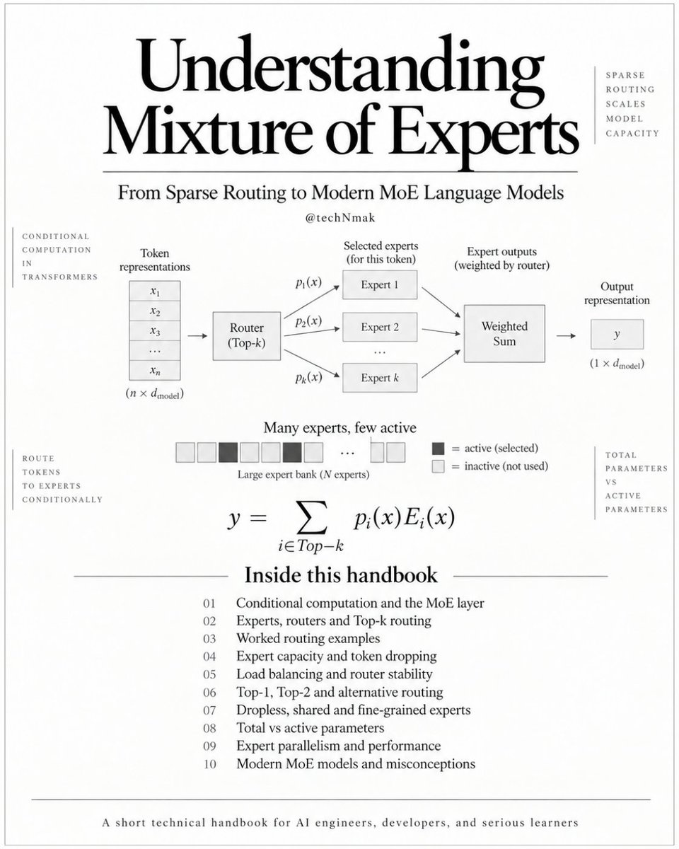
I put together a handbook on how Mixture of Experts actually works, starting with what happens when a Transformer FFN becomes a routed bank of experts and only a small subset is selected for each token.

It works through router logits, Top-k selection, expert weighting, load balancing, capacity and token dropping, router z-loss, dropless execution, total vs. active parameters, expert parallelism, and how these ideas show up in Mixtral, DeepSeek-V3, and Qwen3. Worked examples throughout, with citations back to the original papers and current implementations.

Made it to be the explanation I wish I'd had when I first tried to understand how modern MoE models can grow so large without activating the full expert bank for every token.

[Akshay 🚀 @akshay_pachaar]

13 attention mechanisms AI engineers must know:

(bookmark this)

The tricky part about attention is that these techniques are often discussed together, even though they solve very different problems.

Some reduce KV cache size. Some control which tokens can attend to each other. Others make attention cheaper to compute or improve how KV cache is managed during serving.

So, a better way to organize them is by the bottleneck they actually solve.

Let's do that:

𝟭. 𝗞𝗩 𝗵𝗲𝗮𝗱 𝘀𝗵𝗮𝗿𝗶𝗻𝗴, 𝘄𝗵𝗲𝗻 𝗞𝗩 𝗰𝗮𝗰𝗵𝗲 𝘀𝗶𝘇𝗲 𝗶𝘀 𝘁𝗵𝗲 𝗯𝗼𝘁𝘁𝗹𝗲𝗻𝗲𝗰𝗸

→ MHA (multi-head attention) gives every query head its own key and value heads, providing maximum flexibility but also the largest KV cache.

→ MQA (multi-query attention) makes all query heads share a single KV head, dramatically reducing cache size.

→ GQA (grouped query attention) groups query heads and gives each group a shared KV head, balancing memory savings with model quality.

→ MLA (multi-head latent attention) compresses keys and values into a smaller latent representation before caching them, reducing KV memory even further.

𝟮. 𝗔𝘁𝘁𝗲𝗻𝘁𝗶𝗼𝗻 𝗽𝗮𝘁𝘁𝗲𝗿𝗻𝘀, 𝘄𝗵𝗲𝗻 𝘄𝗵𝗮𝘁 𝘁𝗵𝗲 𝗺𝗼𝗱𝗲𝗹 𝗰𝗮𝗻 𝘀𝗲𝗲 𝗺𝗮𝘁𝘁𝗲𝗿𝘀

→ Causal attention only allows each token to look backward, which is what autoregressive LLMs use for generation.

→ Bidirectional attention lets tokens attend in both directions, which is useful when understanding the entire input at once.

→ Sliding Window Attention restricts each token to nearby context instead of attending across the full sequence.

→ StreamingLLM keeps a small set of anchor tokens plus recent context, allowing generation to continue with bounded memory.

𝟯. 𝗖𝗼𝗺𝗽𝘂𝘁𝗲 𝗲𝗳𝗳𝗶𝗰𝗶𝗲𝗻𝗰𝘆, 𝘄𝗵𝗲𝗻 𝗮𝘁𝘁𝗲𝗻𝘁𝗶𝗼𝗻 𝗶𝘁𝘀𝗲𝗹𝗳 𝗶𝘀 𝗲𝘅𝗽𝗲𝗻𝘀𝗶𝘃𝗲

→ FlashAttention computes exact attention in small tiles that fit in fast on-chip memory, reducing expensive memory movement.

→ Sparse Attention skips selected token-to-token connections entirely, reducing how much attention needs to be computed.

𝟰. 𝗞𝗩 𝘀𝗲𝗿𝘃𝗶𝗻𝗴 𝗲𝗳𝗳𝗶𝗰𝗶𝗲𝗻𝗰𝘆, 𝘄𝗵𝗲𝗻 𝗽𝗿𝗼𝗱𝘂𝗰𝘁𝗶𝗼𝗻 𝘁𝗵𝗿𝗼𝘂𝗴𝗵𝗽𝘂𝘁 𝗶𝘀 𝘁𝗵𝗲 𝗯𝗼𝘁𝘁𝗹𝗲𝗻𝗲𝗰𝗸

→ PagedAttention stores KV cache in blocks allocated on demand, reducing wasted and fragmented GPU memory.

→ RadixAttention organizes shared prefixes so KV states can be reused across requests instead of recomputed.

→ Prefix Caching similarly reuses KV blocks for repeated prefixes such as system prompts, reducing redundant prefill work.

The important part is that these techniques are complementary.

An LLM can use GQA to shrink its KV cache, FlashAttention to compute attention efficiently, Sliding Window Attention to limit context interactions, and PagedAttention to manage that cache efficiently in production.

Once you organize them by the bottleneck they solve, the attention landscape becomes much easier to reason about.

I wrote a deeper breakdown of how these techniques evolved and the problem each one solves.

The full article is quoted below.

Thanks for reading.

Cheers! :)

[Avi Chawla @_avichawla]

One architectural change can cut KV cache by 8x!

In standard multi-head attention, every query head gets its own key and value head.

So a model with 64 query heads therefore stores 64 sets of key and value vectors for every token at every layer.

Multi-query attention optimizes this. It shares one KV head across all query heads. This produces the smallest cache, although that much sharing can reduce model quality.

Grouped-query attention lies between them.

It divides the query heads into groups, with each group sharing one KV head.

In Llama 3 70B, every eight query heads share one KV head. The model stores 8 sets of KV vectors instead of the 64 that an equivalent MHA layout would need.

That makes this part of the KV cache 8x smaller. It also reduces the amount of KV data read during decoding by the same factor, assuming the remaining dimensions and precision stay unchanged.

This is part of the model architecture, so it cannot be enabled on an arbitrary MHA model with a serving flag.

And this is only one way to control KV-cache cost.

I covered GQA alongside 11 other methods in the KV Cache Engineering article. It explains which part of the cost each method reduces and whether it requires a different model architecture or only a serving-engine change.

Read it below.

[Tech with Mak @techNmak]

I thought I understood GPU utilization until I started working on this handbook.

I kept collapsing three different things into one mental picture => the work a kernel launches, the work that is actually resident on the GPU, and the work that is ready to issue right now. They are not the same thing.

Take a kernel with 240 blocks and 256 threads per block. That is 61,440 logical threads, or 1,920 NVIDIA warps. But those warps are not all physically resident at once. Blocks are admitted onto SMs as registers, shared memory, thread limits, warp limits and block limits allow. Even after a warp becomes resident, it may still be waiting on memory, an arithmetic dependency or synchronization. The scheduler can only choose from warps that are actually eligible to issue.

That changed how I read performance numbers too.

Occupancy is a residency number => resident warps compared with the architectural maximum. GPU utilization measures something different. In NVML it is basically the fraction of the sampling window during which at least one kernel was executing.

So a GPU can show 100% utilization without Tensor Cores being saturated, without HBM bandwidth being saturated, and while one subsystem is the bottleneck and large parts of the GPU remain underused.

Memory has the same kind of traps. Registers, shared memory, L1, L2 and HBM are not just increasingly slower boxes. They have different scope, capacity, management and access behavior.

A model fitting in HBM tells you that it fits. It tells you almost nothing about how many bytes move, whether accesses coalesce well, how much reuse you get, or whether memory is what is holding the kernel back.

FlashAttention is a nice example => the dense attention math stays the same, but the execution schedule is reorganized to reduce traffic between HBM and on-chip storage.

Tensor Cores were another thing I had mentally oversimplified. They are specialized matrix multiply-accumulate hardware and they matter enormously for AI, but they do not “run the model.” Reductions, indexing, elementwise work, synchronization, memory movement, launches and plenty of other instructions still go through other parts of the GPU.

After a while I stopped asking "why isn’t the GPU at 100%?" and started asking a better question => what is actually limiting useful progress right now?

That ended up becoming a 42-page handbook.

SMs, warps, schedulers, occupancy, latency hiding, registers, shared memory, caches, HBM, coalescing, Tensor Cores, GEMM mapping, precision, utilization and the performance numbers that are very easy to misread.

Do read.

[Akshay 🚀 @akshay_pachaar]

PagedAttention, clearly explained.

(how vLLM manages KV cache like an operating system)

every request a serving engine handles needs GPU memory for its KV cache, the key and value vectors stored per token so later tokens can attend over the prompt without recomputing it.

the engine has no way to know how many tokens the request will generate.

the simple approach is to reserve one contiguous slab per request based sized for the maximum allowed length (max_token_size).

for example, a request with max_token_size = 4,096 tokens gets 4,096 slots the moment it arrives and holds them until it finishes, even if it stops at 40.

the left side of the graphic below shows what that does to memory.

→ a large part of every slab is reserved but unused. those slots belong to one request until it finishes, and most of them never get written.

→ the grey pieces between slabs are fragmentation gaps. as requests of different sizes come and go, the free memory breaks into fragments that are each too small for a new slab, even when the total free space would fit several requests.

a new request needs a contiguous slab, none of the gaps fit one, and the reserved slots cannot be taken back, so it waits while the GPU holds mostly empty space.

the vLLM team measured 60 to 80% of KV cache memory wasted this way in existing serving systems.

they introduced PagedAttention which is inspired from how operating system uses RAM. instead of one slab per request, the KV cache is handed out in blocks.

a block is a fixed-size chunk of GPU memory that holds the keys and values for a fixed number of consecutive tokens, in vLLM the default value is 16. inside it sits the full KV state for those 16 tokens across every layer and every KV head.

at startup the engine measures the GPU memory left after loading the weights and carves all of it into a pool of numbered physical blocks. that pool is the grid in the graphic below, and it is the only KV memory that will ever exist.

the bottom row shows how a request uses that pool.

→ a request arrives and its sequence is split into logical blocks, L1 for tokens 1 to 16, L2 for 17 to 32, and so on. a logical block is only an index into the sequence, it holds nothing itself.

→ each logical block is assigned a physical block from the pool and the pairing is recorded in the request's block table. the assignment happens only when the previous block fills, so no request holds memory it has not written yet.

→ at each decode step the attention kernel reads the block table and gathers keys and values from whichever physical blocks they landed in. a request's tokens no longer need to be next to each other in memory, which is why consecutive logical blocks can sit at scattered grid positions.

every physical block is the same size, so any free one serves any request and fragmentation gaps stop forming. when a request finishes, its block numbers go straight back to the pool for the next request to take.

waste can never be more than the unfilled tail of a single 16-token block, which is how it drops under 4%. the reclaimed memory becomes batch size, meaning more requests generating at the same time on one GPU.

that is where the 2 to 4x throughput gain comes from. each generation step is limited by how fast the model weights can be read from memory, and a bigger batch spreads that read across more tokens.

the model itself is untouched. whatever attention variant it was trained with runs the same way under PagedAttention, because the change lives entirely in how the serving engine hands out memory.

i wrote the full breakdown of every attention mechanism, from multi-head attention through FlashAttention and sparse attention, up to PagedAttention and RadixAttention.

the article is quoted below.

[Tech with Mak @techNmak]

KV cache is one of the most important ideas in LLM inference, but it is often explained too casually.

During autoregressive generation, a model produces one token at a time. Without caching, each new decoding step would repeatedly recompute key and value states for tokens the model has already processed. KV caching avoids that redundant work by storing those past K/V tensors and reusing them as the sequence grows.

That sounds simple, but it has consequences across the entire serving stack. The cache grows with sequence length, consumes significant GPU memory, creates memory-bandwidth pressure during decoding, and helps explain why architectures moved from MHA to MQA and GQA, why MLA takes a different compression approach, and why systems such as PagedAttention exist in the first place. It also explains why long context is not free, why prefix caching is a separate optimization, and why KV cache should not be confused with an LLM’s memory.

I put together a technical handbook that works through this from first principles => what exactly gets cached, the tensor shapes, the memory formula, concrete MHA/GQA/MQA calculations, prefill vs. decode, MLA, PagedAttention, prefix reuse, offloading, quantization, eviction, and the common misconceptions around all of it.

The explanations are grounded in the original papers and current framework documentation.

Sharing the handbook here

[DeepLearning.AI @DeepLearningAI]

🗑️ AI agents need better garbage collection.

Xiaohongshu researchers built Self-GC, using a planner LLM to decide which context tokens to keep, fold, or prune. In tests, it retained necessary details 84.85 percent of the time compared to just 54.55 percent for standard methods.

Master agent memory management: https://t.co/aEAfkFazQN

#DeepLearningAI #AIAgents #LLMs

[Karan🧋 @kmeanskaran]

INTRODUCING AGENTIC SYSTEM TRILOGY 🔥👀

I created a series of 3 articles, covering:
1. System Design for Agent Systems
🔗 https://t.co/8RNML1fBIJ

2. Designing the Backend for Agent Systems
🔗https://t.co/2vdYYMj7Cv

3. Deployment of Agent Systems to AWS ECS
🔗https://t.co/nJqmCOJ3ak

I made a PoC called agent-harness-ops and deployed to AWS ECS (Repo link in comment).

- Designing harness (memory, context management, human in the loop, etc.)
- Create a production level backend (Cache, rate limit, FastAPI)
- Design queue workers using Celery and Redis
- Set CI/CD using GitHub Actions (pipelines, dev/prod environments, tag release)
- Use AWS services (DynamoDB, ECR, ECS, ALB, Bedrock models)
- Set up Terraform for dev and prod enviroment
- Trace logs, observability, AWS CloudWatch
- Automate complete system with best practices
And much more.

This trilogy make sure you will learn real-time production system and no more toy projects.

Open for feedbacks :)

[Tom Yeh @ProfTomYeh]

Autoencoder by hand ✍️ interactive diagram. Open https://t.co/FG7rsyXRyG

[Avi Chawla @_avichawla]

Why KV cache stores K and V vectors but never Q?

(a popular technical LLM interview question)

LLMs are autoregressive so each token is predicted from every token before it, one at a time.

This autoregressive nature has a direct consequence inside the model.

A forward pass over <n> tokens produces <n> hidden states, but only the last one is projected to logits and is required to generate the next token.

So to understand why KV cache just stores K and V vector, we must back track to see how exactly is the last hidden state produced.

Let's walk through this with a 10-token prompt.

1) Prefill:

All 10 tokens go through the model in one forward pass, in parallel (with causal masking), since the whole prompt is already known.

At every layer, each of the 10 positions produces a query, a key and a value vector, and attention at each position runs against all positions up to it.

This pass is compute-heavy, and it's why the first token takes noticeably longer than the ones after it. TTFT is mostly prefill.

2) The first output token:

To generate the 11th token, only the 10th token's hidden state is needed. So this is projected from the hidden-dim to vocab-dim to generate logits over vocab.

These logits then go through softmax and sampling to generate token 11.

3) Back-track the hidden state:

The last hidden state is the last row of the feedforward block's output. The feedforward block is position-wise (it's applied to each row independently) so that row comes from the last row of the attention output before it.

So now we need to see how the last row of attention is computed.

4) Attention matrix:

QKᵀ for a 10-token prompt will give a 10 × 10 matrix.

Row <i> will have the dot product of query <i> with every key.

Row 10 is therefore Q₁₀·K₁, Q₁₀·K₂, all the way to Q₁₀·K₁₀.

Notice that only Q₁₀ appears in it. Q₁ through Q₉ only belong to their corresponding rows 1-9, and those rows' hidden states we already discarded because they were never needed.

The last row of attention goes through softmax and multiplies the full stack of value vectors, V₁ through V₁₀, to give the last row of the attention output.

So the last hidden state depends on exactly three things: Q₁₀, every key, and every value.

5) Generating token 12:

Token 11 is appended, and this time, we need row 11's hidden state to generate token 12.

Mathematically, attention operation turns out to be Q₁₁ against K₁ through K₁₁, then multiplied by V₁ through V₁₁.

K₁ through K₁₁ and V₁ through V₁₁ are bit-for-bit what prefill + first token produced since under causal masking, a token's key and value depend on that token and the ones before it, never on anything after, so appending token 11 cannot change anything at position 3.

6) The cache state:

Overall, this implies that you just need to retain the keys and values at each decoding step, and compute only the new position's Q, K and V.

Each decode step requires one query vector, which is never used again, so they are never cached across the decoding process.

The visual below explains the entire process.

That said, KV cache is only one of four separate caching layers in an LLM stack.

The other three are prefix caching on the server, prompt caching billed by a provider, and a semantic cache that skips the model entirely.

I wrote a full breakdown of all four caches in LLM serving that you should know as an AI engineer, with code for each.

Read it below.

[Daily Dose of Data Science @DailyDoseOfDS_]

CPU vs GPU vs TPU vs NPU vs LPU, explained visually:

5 hardware architectures power AI today.

Each one makes a fundamentally different tradeoff between flexibility, parallelism, and memory access.

> CPU

It is built for general-purpose computing. A few powerful cores handle complex logic, branching, and system-level tasks.

It has deep cache hierarchies and off-chip main memory (DRAM). It's great for operating systems, databases, and decision-heavy code, but not that great for repetitive math like matrix multiplications.

> GPU

Instead of a few powerful cores, GPUs spread work across thousands of smaller cores that all execute the same instruction on different data.

This is why GPUs dominate AI training. The parallelism maps directly to the kind of math neural networks need.

> TPU

They go one step further with specialization.

The core compute unit is a grid of multiply-accumulate (MAC) units where data flows through in a wave pattern.

Weights enter from one side, activations from the other, and partial results propagate without going back to memory each time.

The entire execution is compiler-controlled, not hardware-scheduled. Google designed TPUs specifically for neural network workloads.

> NPU

This is an edge-optimized variant.

The architecture is built around a Neural Compute Engine packed with MAC arrays and on-chip SRAM, but instead of high-bandwidth memory (HBM), NPUs use low-power system memory.

The design goal is to run inference at single-digit watt power budgets, like smartphones, wearables, and IoT devices.

Apple Neural Engine and Intel's NPU follow this pattern.

> LPU (Language Processing Unit)

This is the newest entrant, by Groq.

The architecture removes off-chip memory from the critical path entirely. All weight storage lives in on-chip SRAM.

Execution is fully deterministic and compiler-scheduled, which means zero cache misses and zero runtime scheduling overhead.

The tradeoff is that it provides limited memory per chip, which means you need hundreds of chips linked together to serve a single large model. But the latency advantage is real.

AI compute has evolved from general-purpose flexibility (CPU) to extreme specialization (LPU). Each step trades some level of generality for efficiency.

The visual below maps the internal architecture of all five side by side.

Notice the thread connecting all five. Every generation exists to move data less, because the math was never the hard part. Feeding the math units fast enough is.

The same battle plays out one layer up in software. During LLM inference, a single GPU produces terabytes of KV cache per day, and nearly all of it gets thrown away and recomputed, which is a big reason agent workloads cost what they do.

We wrote a full breakdown of how a disaggregated caching layer fixes this, with up to 14x faster time-to-first-token. The article is quoted below.

You should also check the LMCache GitHub repo: https://t.co/VCPBztdMhP

(don't forget to star 🌟)

👉 Over to you: Which of these 5 have you actually worked with or deployed on?

[Avi Chawla @_avichawla]

A harnessed LLM agent, clearly explained!

Two agents can run the same model on the same task and finish as expected. But one of them can spend nearly 3x the tokens to complete the task.

The extra usage originates from the code wrapped around them, which decides what reaches the model's context on each call and how many calls there are.

For instance, consider a tool that returned 50k tokens of JSON at some step. If it stays in the context, the model will continue to read that payload again at every subsequent step.

Tool definitions behave the same way.

A server can expose 50 tools, each with a name, a description, and an input and output schema.

By default, all of them will stay in the prompt from the first call, whether the agent uses them or not.

However, an optimally built harness can avoid that unnecessary cognitive load on the model.

More specifically, one core design principle of harness engineering is to push things out of the model at the right time:

- Memory holds the state that weights and context shouldn't carry.
- Skills hold procedural knowledge. These cover the operating procedures and heuristics that specialize a general model.
- Protocols hold the interaction contracts for users, other agents, and tools.

Do note that the context never disappears permanently.

It is always loaded when needed, and the harness decides how much is loaded and when.

For instance, to manage a 50k token payload, a harness can write it to a file and keep a preview and a path in context, hand the work to a subagent whose context is discarded afterwards, or summarize the older messages once the conversation passes a threshold.

If you want to see this in practice, TrueForge is an open-source harness that already implements these practices.

Tool schemas are deferred unless preloading is switched on, large responses go to a sandbox file, and generated code calls tools back through the harness, so the sandbox never holds the credentials.

The two agents I talked about at the top are from DevRev's Enterprise-Bench. TrueForge solved the same number of tasks as Claude Managed Agents on the same model, using a bit over a third of the tokens and around 40% fewer tool calls.

Here's the GitHub repo: https://t.co/ZjePhhfKIh

(don't forget to star it ⭐ )

I also wrote a full breakdown of where agent tokens actually go inside a run, covering context accounting, the strategies above, and the benchmark in detail, and TrueForge worked with me to put this together.

Read it below.

[Tom Yeh @ProfTomYeh]

CLIP by hand ✍️ ~ 13 steps walkthrough below

CLIP, Contrastive Language-Image Pre-training, is OpenAI's answer to a question that sounds impossible: how do you put a sentence and a picture in the same space?

CLIP shipped when OpenAI was still open, and those embeddings were shared far and wide. Almost every multimodal model you use today descends from them.

How does it work?

Goal: learn one shared embedding space for text and images.

= 1. Given =

A mini batch of three text-image pairs. OpenAI trained the original on 400 million.

= 2. Text to vectors =

Let us look up each word with word2vec.

= 3. Image to vectors =

We cut each image into two patches and flatten them. Now text and pixels are both just numbers.

= 4. The other pairs =

Repeat steps 2 and 3 for the rest of the batch.

= 5. Encode =

Let us push both sides through their encoders, a linear layer and a ReLU. In practice these are transformers, but the shape of the operation is the same.

= 6. Mean pooling =

We average across the columns, so each image and each sentence collapses to a single vector.

= 7. Projection =

The text vectors are 3D and the image vectors are 4D, so they cannot be compared at all. A linear layer projects both to 2D. That 2D space is the shared embedding space, and getting here is the whole point of the model.

= 8. Prepare for matmul =

Let us copy the text vectors down and the transposed image vectors across.

= 9. MatMul =

We multiply, which takes the dot product of every text vector with every image vector. Each cell is one estimate of how well a sentence matches a picture.

= 10. Softmax, e to the power =

Raise e to each cell. To keep it hand sized we approximate e with 3.

= 11. Softmax, sum =

Sum each row for image to text, each column for text to image.

= 12. Softmax, normalize =

Divide, and out come two similarity matrices, one per direction.

= 13. Loss gradients =

The targets are identity matrices: a pair that belongs together should score 1, every other cell 0. Subtract the target from the similarity and you have the gradients, in both directions.

The takeaway: pairing a picture with a sentence comes down to a single dot product. Everything before step 9 is the work of getting them into one shared space, so that the dot product finally means something.

💾 Save this post!

[Roan @RohOnChain]

Don't waste 2 years learning to become an AI agentic engineer in 2026.

Andrew Ng, the godfather of AI, gave the complete playbook to become one from scratch.

1 hour course. Free:

• 00:00 - AI agent basics
• 12:12 - AI Agentic workflows & design patterns
• 53:27 - Practical tips for building AI agents
• 1:20:30 - self-improving AI agent loops
• 1:30:19 - multi-agent AI systems

I watched it last night.

Halfway through, I realized I could get into Anthropic in weeks, not years.

Bookmark now. Watch it. Then build your own AI agent with the guide below.

[Daily Dose of Data Science @DailyDoseOfDS_]

Claude Code’s architecture, explained visually:

(bookmark this)

Claude Code is a lot more than a CLI that invokes the Claude models.

The actual system has six layers, and the model is just one node inside the loop.

The diagram below explains every component:

1) Input layer handles session management, permission gating, and YAML-based trust tiers before anything reaches the model.

2) Knowledge layer holds the skill registry, context compressor, task graph, and cross-session memory store. This is where harness intelligence lives outside the weights.

The context compressor is a 5-layer cascade that kicks in when the context window hits roughly 95% capacity. It doesn’t summarize your conversation the way ChatGPT does. Instead, it runs structured extraction on file paths, code snippets, and error histories while pruning redundant tool outputs. The goal is to keep the context usable, not just smaller.

3) Execution layer runs tool dispatch through a typed registry with one handler per tool, like bash, read, write, grep, glob, and revert.

The streaming runtime handles parallel execution, and the prompt cache reuses stable prefixes at roughly 10% of the original cost.

4) Integration layer connects the MCP runtime to external servers (filesystem, git, custom). Tools register inward, and memory writes outward to a markdown file (agent_memory.md) that persists across sessions.

5) Multi-agent layer is the most underappreciated piece, and it works very differently from what most people assume.

Claude Code supports two levels of parallelism:

- Subagents are lightweight workers that run inside your session. They get their own context window, do a focused task (search the codebase, explore a file tree), and return results to the parent. They can’t talk to each other, and they can’t spawn their own subagents. It’s a strict parent-child hierarchy.

- Agent teams go further. One session acts as a team lead, and it spawns independent teammates, each running as a full Claude Code instance with its own context window. The team lead breaks a task into subtasks, assigns them, and monitors progress.

The coordination happens through two mechanisms → a shared task list (JSON files on disk) and a mailbox system for peer-to-peer messaging.

Each teammate gets git worktree isolation. It’s a separate working directory with its own branch, sharing the same repository history.

This means agents can write to overlapping parts of the codebase without file conflicts. When they finish, worktrees with no changes are cleaned up automatically. Worktrees with changes persist for human review before merging.

6) Observability layer wraps everything. An event bus with lifecycle hooks logs all tool calls and messages, creating a complete audit trail of the agent’s actions and decisions.

Background executors run daemon threads non-blocking, so observability never stalls the main loop.

Finally, the master agent loop sits at the center of all six layers. It assembles context, calls the model, receives a tool request, executes it, feeds the result back in, and repeats. Every iteration is one turn.

Within a turn, the model might request a tool call. That request flows through the permission system, gets executed, and the output feeds back into the loop as the next input.

The loop itself is single-threaded on purpose. All the intelligence lives in the layers around it, not in the loop logic. Anthropic calls it a dumb loop because the model reasons, and the harness mediates.

This is the architecture behind Claude Code.

If you want to dive deeper into Claude Sugagents and agent teams specifically, we wrote an article about them.

It explains the difference between Claude sub-agents (isolated, fire-and-forget workers) and agent teams (persistent, peer-communicating instances with a shared task list), and when to use each.

Read it below.

[Avi Chawla @_avichawla]

From prompt → context → harness → loop → graph engineering:

The list keeps growing, and every new term gets treated as a replacement for the last one.

In reality, however, each layer wraps the one before it, and the cleanest way to tell them apart is to ask what a single unit of work looks like.

> Prompt engineering is the message:

The model remembers nothing before this call, so the prompt has to carry the full universe of what it needs. a role, the background, the instructions, a few examples, and a format.

When the output falls short, the skill is working out which ingredient lets you down, not rewriting the instructions every time.

The unit of work is one input.

> Context engineering is the memory:

Across many steps, the window is finite, and the available information is not, which forces a curation step. A curator keeps what matters, compresses what is useful but bulky, and drops the rest.

Good curation is mostly about knowing what to throw away, not packing more in.

The unit of work is what stays in the window.

> Harness engineering is the machine:

On its own, a model just generates text. The harness gathers what it needs, runs it, calls tools or sub-agents, and verifies the result with tests or a judge.

That verify step is the entire difference between calling an api and running an agent.

The unit of work is one pass through the machine.

> Loop engineering is the run:

One pass rarely finishes the job, so something has to decide whether to run the machine again. That decision needs a goal defined upfront, brakes like max iterations and budget caps, and a completion check that is automated rather than felt.

An agent that stops asking for tools has ended its turn, which is not the same as finishing the task.

The unit of work is the whole run.

> Graph engineering is the coordination:

Once several loops have to work together, you need to say what runs when, what runs in parallel, and who checks whom. Nodes do the work, edges decide what runs next, and shared state flows between them.

A single loop is just a one-node graph with an edge pointing back at itself, which is why graphs govern loops instead of replacing them.

The unit of work is the whole job.

Here is the part that ties it together.

Prompt and context both live inside the harness gather step. The harness is one pass, the loop decides whether to run that pass again, and the graph decides which loops run at all.

Zoom out, and the unit of work gets bigger. Zoom in, and you are back at the prompt.

That also tells you where to debug. Find the layer whose unit of work broke, then fix that layer.

The prompt is the easiest layer to edit, which is why it keeps taking the blame for failures that live three layers up.

My co-founder published a deep dive on graph engineering, covering the core idea, how to get started, shared state, routing you can trust, and when a graph is genuinely overkill.

Read it below.

[Kunal Bhashkar @BhashkarKunal]

:)

[Avi Chawla @_avichawla]

11 LLM evaluation methods AI engineers must know:

(bookmark this)

Two eval metrics can rank the same two models in opposite orders, and neither one is wrong.

A model that paraphrases the reference can score near zero on BLEU and near the top on BERTScore for the exact same output.

Neither metric is wrong because one is measuring wording and the other is capturing meaning.

This is why LLM evaluation is fragmented into several methods, depicted in the visual below and grouped by what each one assumes:

> Reference-based (ground truth exists):

- BLEU
- ROUGE
- BERTScore

> Judge-based (no ground truth):

- G-Eval
- LLM-as-Judge
- LLM juries

> Human and deterministic:

- Human eval
- DAG

> Built for agents:

- Trajectory accuracy
- Multi-turn eval

> Run as a gate:

- Safety eval

To use them in practice, most of these metrics are already implemented in Opik, which is open source (20k+ stars) and runs them over traced production data. You can start using them in a few lines of code.

GitHub repo: https://t.co/vahjkkfJCt

(don’t forget to star it ⭐️)

That said, metrics only point at the failing case.

The rest of the work is still done manually, like inspecting the trace to see where the span went wrong, editing a prompt or a tool description, re-running, and checking that the fix did not break anything else.

My co-founder wrote a walkthrough (with code) that automates this loop using Opik.

It explains the full lifecycle where a failing trace gets diagnosed, the fix runs against the exact input that failed, and that input stays in the eval set as a regression case so it does not recur.

Read it below.