Deepak Pachaar

[Akshay 🚀 @akshay_pachaar]

13 attention mechanisms AI engineers must know:

(bookmark this)

The tricky part about attention is that these techniques are often discussed together, even though they solve very different problems.

Some reduce KV cache size. Some control which tokens can attend to each other. Others make attention cheaper to compute or improve how KV cache is managed during serving.

So, a better way to organize them is by the bottleneck they actually solve.

Let's do that:

𝟭. 𝗞𝗩 𝗵𝗲𝗮𝗱 𝘀𝗵𝗮𝗿𝗶𝗻𝗴, 𝘄𝗵𝗲𝗻 𝗞𝗩 𝗰𝗮𝗰𝗵𝗲 𝘀𝗶𝘇𝗲 𝗶𝘀 𝘁𝗵𝗲 𝗯𝗼𝘁𝘁𝗹𝗲𝗻𝗲𝗰𝗸

→ MHA (multi-head attention) gives every query head its own key and value heads, providing maximum flexibility but also the largest KV cache.

→ MQA (multi-query attention) makes all query heads share a single KV head, dramatically reducing cache size.

→ GQA (grouped query attention) groups query heads and gives each group a shared KV head, balancing memory savings with model quality.

→ MLA (multi-head latent attention) compresses keys and values into a smaller latent representation before caching them, reducing KV memory even further.

𝟮. 𝗔𝘁𝘁𝗲𝗻𝘁𝗶𝗼𝗻 𝗽𝗮𝘁𝘁𝗲𝗿𝗻𝘀, 𝘄𝗵𝗲𝗻 𝘄𝗵𝗮𝘁 𝘁𝗵𝗲 𝗺𝗼𝗱𝗲𝗹 𝗰𝗮𝗻 𝘀𝗲𝗲 𝗺𝗮𝘁𝘁𝗲𝗿𝘀

→ Causal attention only allows each token to look backward, which is what autoregressive LLMs use for generation.

→ Bidirectional attention lets tokens attend in both directions, which is useful when understanding the entire input at once.

→ Sliding Window Attention restricts each token to nearby context instead of attending across the full sequence.

→ StreamingLLM keeps a small set of anchor tokens plus recent context, allowing generation to continue with bounded memory.

𝟯. 𝗖𝗼𝗺𝗽𝘂𝘁𝗲 𝗲𝗳𝗳𝗶𝗰𝗶𝗲𝗻𝗰𝘆, 𝘄𝗵𝗲𝗻 𝗮𝘁𝘁𝗲𝗻𝘁𝗶𝗼𝗻 𝗶𝘁𝘀𝗲𝗹𝗳 𝗶𝘀 𝗲𝘅𝗽𝗲𝗻𝘀𝗶𝘃𝗲

→ FlashAttention computes exact attention in small tiles that fit in fast on-chip memory, reducing expensive memory movement.

→ Sparse Attention skips selected token-to-token connections entirely, reducing how much attention needs to be computed.

𝟰. 𝗞𝗩 𝘀𝗲𝗿𝘃𝗶𝗻𝗴 𝗲𝗳𝗳𝗶𝗰𝗶𝗲𝗻𝗰𝘆, 𝘄𝗵𝗲𝗻 𝗽𝗿𝗼𝗱𝘂𝗰𝘁𝗶𝗼𝗻 𝘁𝗵𝗿𝗼𝘂𝗴𝗵𝗽𝘂𝘁 𝗶𝘀 𝘁𝗵𝗲 𝗯𝗼𝘁𝘁𝗹𝗲𝗻𝗲𝗰𝗸

→ PagedAttention stores KV cache in blocks allocated on demand, reducing wasted and fragmented GPU memory.

→ RadixAttention organizes shared prefixes so KV states can be reused across requests instead of recomputed.

→ Prefix Caching similarly reuses KV blocks for repeated prefixes such as system prompts, reducing redundant prefill work.

The important part is that these techniques are complementary.

An LLM can use GQA to shrink its KV cache, FlashAttention to compute attention efficiently, Sliding Window Attention to limit context interactions, and PagedAttention to manage that cache efficiently in production.

Once you organize them by the bottleneck they solve, the attention landscape becomes much easier to reason about.

I wrote a deeper breakdown of how these techniques evolved and the problem each one solves.

The full article is quoted below.

Thanks for reading.

Cheers! :)

[Ministry of Education @EduMinOfIndia]

From classrooms to school corridors, students are stepping up as Waste Warriors—segregating waste, making responsible choices and turning cleanliness into a daily habit.

Through Eco Clubs for Mission LiFE, Department of School Education and Literacy, is sensiting young learners to the Solid Waste Management Rules 2026 so that they understand the importance of segregation and the 5Rs- refuse, reduce, reuse, repurpose and recycle waste.

#SBMG, #SWMRules2026
#SwachhBharat #LifestyleForEnvironment #EcoClubsforMissionLiFE #SchoolEducation #DoSEL

[Akshay 🚀 @akshay_pachaar]

Researchers found a surprisingly simple path to 82% fewer LLM errors.

Instead of searching for one universally best model, they combined the strengths of many.

21 LLMs were evaluated across 16 benchmarks, running every model 10 times on each prompt.

Different models failed on different problems. Even the same model could fail once and succeed on another attempt.

So they calculated what happens when the optimal model is selected for every prompt.

At matched cost, this reduced the average error rate by 54% compared with the best individual model.

It also matched SOTA quality at 85% lower cost.

With up to 10 answers and a perfect judge selecting the best one, the error reduction reached 82%.

Model routing itself is not new.

What is new is measuring its true ceiling while correcting the statistical bias created by selecting lucky results from noisy runs.

Production routers do not select perfectly today and this research reveals how much performance existing models may already contain when used together.

Martian also turned the research into AI Frontier, an interactive dashboard for exploring the results, and I worked with their team today.

More details below.

[Akshay 🚀 @akshay_pachaar]

The easiest way to find out which models you can run on your computer:

Just run:

- 𝗻𝗽𝗺 𝗶 -𝗴 @𝗺𝗮𝗴𝗻𝗶𝘁𝘂𝗱𝗲𝗱𝗲𝘃/𝗰𝗹𝗶
- 𝗺𝗮𝗴𝗻𝗶𝘁𝘂𝗱𝗲 𝘀𝗲𝘁𝘂𝗽

It profiles your machine and ranks the models across:

- Speed
- Accuracy
- Intelligence
- Memory required

Finally, you can choose your favorite harness (Pi, OpenCode, Claude Code, Codex, etc.) to run with it.

Get started here: https://t.co/gpwU34NFlw

(don't forget to star 🌟)

I also wrote a detailed article on running your favorite harnesses with local models. The article is quoted below.

[Akshay 🚀 @akshay_pachaar]

https://t.co/y0RliaWgqT

[Akshay 🚀 @akshay_pachaar]

run agent harnesses 100% private & offline.

(no token costs, no API keys, 100% open-source)

your agent runs locally. the model doesn't. every prompt, every file, and every secret still leaves your machine before the agent does anything with it.

Magnitude fixes that. it's an open source inference server that runs models on your own hardware and plugs into the coding agent you already use.

setup is one command. it profiles your machine, measures the memory bandwidth that sets your token rate, and hands back complete configurations instead of a list of models. each one names a model, a compression level, a context size, and a speed range you can expect. pick one and start working.

it doesn't replace your harness. setup asks which one you want and writes that config for you. Pi, OpenCode, Claude Code, Codex, and Cline all work, and there's a built-in one tuned for local models if you don't have a harness yet.

that one uses your shell, edits files, and runs scripts out of the box. add skills and it handles Excel, PowerPoint, PDFs, or Chrome.

everyday work it covers:

→ analyze sensitive data
→ manage private notes
→ review code and logs
→ search and organize files
→ build docs or slides

Apache 2.0. no rate limits, and nothing leaves the machine.

𝗻𝗽𝗺 𝗶 -𝗴 @𝗺𝗮𝗴𝗻𝗶𝘁𝘂𝗱𝗲𝗱𝗲𝘃/𝗰𝗹𝗶

the repo is here: https://t.co/gpwU34NFlw

(don't forget to star 🌟)

i wrote the full breakdown of why picking the configuration is the hard part. the article is quoted below.

[KV IIT JODHPUR @kviitjodhpur]

केंद्रीय विद्यालय आईआईटी जोधपुर में प्राचार्य महोदय द्वारा हिंदी माह का शुभारंभ किया गया। इस अवसर पर हिंदी भाषा के महत्व को रेखांकित करते हुए हिंदी के अधिकाधिक प्रयोग एवं प्रचार-प्रसार का संदेश दिया गया।
हिंदी—हमारी पहचान, हमारी शान! 🇮🇳
@KVS_HQ @EduMinOfIndia @kvsrojaipur

[Akshay 🚀 @akshay_pachaar]

Kubernetes meets LLM inference.

Google, NVIDIA, IBM, and Red Hat are all backing the same open-source project to make it work.

the problem is that LLM inference does not scale the way normal web services do, and the usual Kubernetes answer makes it worse.

let me explain:

run one vLLM or SGLang server and the KV cache is a clean win. the server keeps the attention keys and values for tokens it has already processed, so a prompt that shares a prefix with an earlier one skips past that computation and starts generating.

put a standard Kubernetes Service in front of several replicas and that saving mostly evaporates. the Service hands each request to whichever pod is next in rotation, and that pod usually never saw the prefix, so it recomputes the entire context from scratch.

round-robin assumes every replica serves every request equally well. true for stateless web traffic. false the moment prefill caching exists, because replicas now differ by what they remember.

teaching Kubernetes that difference turns into four problems.

→ knowing which replica holds the prefix. each server streams an event every time it creates or evicts a cache block, and the router keeps a live index of who holds what.

→ knowing when to ignore that index. cache affinity pulls traffic onto warm replicas, so past a load threshold the router drops affinity and picks on load alone. otherwise the warm replica turns into the bottleneck.

→ extending where the cache lives. accelerator memory fills fast, so blocks spill to CPU memory and then disk. on four H100s at 250 concurrent users, that hierarchy delivered 13.9x the throughput of keeping everything on the GPU.

→ separating prefill from decode. prefill is compute-bound, decode is memory-bandwidth-bound, and running both on one replica underuses each. AWS measured up to 70% higher tokens per second after splitting them onto dedicated pools, though the KV cache now has to cross the network before the first token appears.

the KV cache stops being something a single server manages. it becomes cluster state, and the routing layer has to track it.

solve that and you get roughly 3x the output throughput and half the time to first token, on the same hardware, running the same model.

llm-d is the project handling all four on Kubernetes. it sits above vLLM and SGLang rather than replacing them, so you keep whichever engine you already run and it takes over the routing, the cache index, the offloading, and the prefill/decode split. Apache 2.0, CNCF sandbox, with Tesla, Snowflake, Cohere and DigitalOcean running it.

check it out on GitHub: https://t.co/IX1vW7phsj

i wrote the full breakdown of how inference works underneath all of this. the article is quoted below.

[Ministry of Education @EduMinOfIndia]

A green school campus sets the right tone for learning! It also encourages children to love and care for the environment…

Let’s listen to what Hansika has to say 👇

[Akshay 🚀 @akshay_pachaar]

how do you know whether your GPU is compute-bound or memory-bound?

here's a simple explanation:

your model weights sit in HBM (high bandwidth memory), the large pool of memory on the GPU board. no arithmetic happens there.

before any multiplication can run, those weights have to travel from HBM into the arithmetic units, and that trip is the slowest thing the chip does.

so the real question is how much work you get out of each weight once it has made the trip.

that gives you one ratio. count how many arithmetic operations something performs, then count how many bytes it pulled out of HBM to perform them.

divide the first by the second and you get its work per byte, which is the horizontal axis in the visual.

every chip has a break-even value for that ratio, and it is just peak arithmetic divided by peak memory bandwidth.

take an H100. it performs 989 trillion operations per second at 16-bit precision, and it can pull 3.35 trillion bytes per second out of memory.

divide one by the other and you get 295 operations per byte, which is the 300 marked on the chart below.

that number says the chip can afford about 300 operations for every byte it fetches. anything cheaper leaves the arithmetic units idle, waiting on the next delivery.

generating one token for a single request sits at the far left of the red line. every weight is fetched from HBM, gets one multiply and one add (2 operations), and is then dropped.

each weight takes two bytes at 16-bit precision, so that is one operation per byte, roughly 300 times below break-even.

this is why the red segment slopes. along it your speed is set entirely by how fast bytes arrive, so a chip with more arithmetic capability buys you nothing.

batching is how you move right. run 32 requests together and each weight, fetched exactly once, does its multiply and add against 32 different values before being dropped.

the traffic out of HBM is unchanged, and the work you got from it went up 32 times.

a long prompt does the same thing, except the many values come from the tokens of one sequence instead of separate requests.

past the break-even point the line goes flat, which is the green region. processing a long prompt and training both land there, since each fetched byte now feeds enough operations that the arithmetic units become the slow stage and the memory path has capacity to spare.

so the two halves ask for opposite fixes. left of the line you cut bytes moved or reuse each fetch harder, and right of it you need faster arithmetic or better algorithms.

the threshold belongs to the hardware. where your workload sits relative to it belongs to you.

I wrote the full breakdown of how a modern GPU works, and the article is quoted below.

stay tuned for more on this!

[Akshay 🚀 @akshay_pachaar]

Jeff Dean's new company already has competition.

Jeff Dean's Discovery Loop targets one key bottleneck with research today, i.e, research is human-intensive and runs one step at a time.

His argument is that automating the full cycle raises both the count and the quality of experiments, starting with ML research itself.

Transformer Lab's Primus is built around a similar premise, with the research question as the only thing a human provides.

It runs for roughly a day and returns a complete paper.

The loop runs in six stages:

- Literature review: reads and synthesizes existing work before designing anything
- Experiment design: scopes the study, picks models, datasets, and metrics
- Provisioning: brings up GPUs and schedules the jobs
- Execution: runs training and evaluation, catches failures, and retries
- Analysis: checks results against the design it committed to
- Writeup: produces the paper with methodology, findings, and caveats

Each stage on its own is usually a routine task, since agents already do all of them.

But holding them together across a day of wall-clock time wasn't solved yet, since a crash after a few hours invalidates everything after it.

That is a scheduling and state problem more than a model problem.

I tested Primus on a quantization research question, asking it to compare INT8 and FP16 on a small open-source vision model and pick the better tradeoff for consumer GPU deployment.

The video below shows the run and the paper it came back with.

Try it yourself here: https://t.co/RypZlREg7y

In my own run, as it worked, it caught two problems on its own.

The image set it first downloaded was a compressed copy, and the compression was quietly inflating accuracy by about 2.9 points on all three models, so it went back and rebuilt every result on the original photos.

It then noticed its own timing was unfair, since running the two precisions one after the other favoured INT8 at three of the four batch sizes, and switched to alternating them in short blocks.

The result I would not have thought to look for is that INT8 costs ResNet-50 only 0.05 points of accuracy, which looks free, while quietly changing the answer on 4.3 percent of images.

To know whether 4.3 percent was even a lot, it first built the same model twice in FP16 and measured how much two identical builds disagree with each other, which is 0.14 percent.

Nobody has published that baseline, so there was never anything to compare against.

[Akshay 🚀 @akshay_pachaar]

https://t.co/th3W7Li0gz

[Ministry of Education @EduMinOfIndia]

"Towards a Tobacco-Free Generation: The School Rally Challenge" launched nationwide by Department of School Education & Literacy, Ministry of Education, on June 11, 2025. Aims at raising awareness among school students about the harmful effects of tobacco and substance abuse.

Highlights:

• 17,000+ schools participated across 545 districts in 36 States/UTs.
• Student-led activities strengthened the implementation of #ToFEI.
• Winning schools were felicitated on 29 May 2026.
• #NashaMuktVidyalaya Portal was launched to implement DoSEL's Three-Year Action Plan (2026–2029) towards #NashaMuktBharat.

#SchoolEducation #DoSEL

[Ministry of Education @EduMinOfIndia]

Ministry of Education is advancing the vision of #NEP2020 through ULLAS – Nav Bharat Saaksharta Karyakram by enabling adults to acquire foundational literacy, numeracy and essential life skills through the power of volunteerism and community participation.

Become a Volunteer Teacher by registering through the #ULLAS Mobile App and contribute to building a जन-जन साक्षर भारत!

#Education4All #DoSEL #ShikshitBharatViksitBharat #janjansaakshar
#fullliteracy

@PMOIndia @narendramodi @dpradhanbjp @PIB_India @airnewsalerts

[Akshay 🚀 @akshay_pachaar]

Karpathy said something you'll regret ignoring:

"You are still responsible for your software, just as before. You are not allowed to introduce vulnerabilities because of vibe coding. "

He said it while drawing the line between vibe coding and agentic engineering. Agents write more of the code now, but none of that takes the responsibility off you.

The assumption underneath that is that a careful enough reader catches the problem. But some failures don't show up in anything there is to read.

For instance, a common fear with a RAG agent is that it could hallucinate when a question asks something outside its corpus.

But such cases are actually well handled by any competent model now. If nothing in the retrieved context looks relevant, there's no material to build an answer on.

Instead, the majority of failures originate when the retrieved context has partial coverage.

The retrieval pipeline returns context that's topically correct but doesn't cover the full question, and the model completes the remainder from parametric knowledge.

There are no token-level labels in the output to tell what was generated using retrieved context and what came from weights.

Both are streamed the same way.

Detecting this for production-grade apps needs a metric written for it, one that's also aligned with principles of agentic engineering.

And the solution is actually implemented in the eval skill that comes with Google’s Agents CLI.

I described the concern to Claude Code in plain English. It read the agent's code, came back with a plan I approved.

It then reported that no built-in metric isolates the behaviour and wrote a custom rubric called corpus_abstention.

It assigned a single categorical verdict per case rather than aggregating everything into one score, since the built-in raters regenerate their rubrics each run and leave no stable number to trend.

→ GROUNDED_ANSWER
→ CORRECT_ABSTENTION
→ UNGROUNDED_ANSWER (answered entirely from outside knowledge)
→ MIXED_LEAKAGE (grounded, but slips in one unsupported claim)
→ WRONG_ABSTENTION (refused something the docs actually covered)

After this, it automatically generated 33 scenarios partitioned by where the failure could occur, like:

- in-corpus
- off-domain
- out-of-corpus but plausibly answerable
- boundary cases where the topic is covered, but a specific detail isn't.

The baseline score was 19 of 33.
- Off-domain passed 3 of 3, as expected.
- But 6 of 15 in-corpus cases retrieved the right document, cited it correctly, answered accurately, and added a claim the source never made.

The root cause was one line in the agent's instruction: "If you already know the answer to a simple question and no document lookup is needed, you may respond directly without citations."

The eval skill helped flag this, and then Claude removed it and forced retrieval on every question.

This took the suite to 30 of 33, and ungrounded answers went from 6 to 0.

The full recording of my run is below, and I worked with the Google Cloud team on this.

Agents CLI GitHub repo → https://t.co/p2WQYblUvX

(don't forget to star 🌟)

I wrote up the full build covering all six steps from install to enterprise registration.

It includes the eval scorecard, the instruction loophole the eval caught before deployment, and what the deployment process actually looks like end-to-end.

Read it below.

[Akshay 🚀 @akshay_pachaar]

Agents that search more, reason less.

(+ a strategy to cut token bills by 76%)

Here's a pattern that shows up in almost every agent trace: the model runs a search, gets backlinks and thirty-word snippets, and then has to go read the web itself.

That means fetching the pages, stripping the markup, and digging out the usable text. All of it happens inside the context window, billed as tokens, before any actual reasoning starts.

That work has a name: the retrieval tax.

On one query it's easy to ignore. In a task that takes several searches, the tax gets paid on every single one, because each new hop re-sends the entire growing context.

To measure it, I did a deliberately simple experiment. I took a question the model already knows from training, "What was Y2K?", so the thinking cost stays fixed and everything above it is pure retrieval overhead.

Answering from memory took about 600 tokens. That's the baseline.

A web search loop took about 3,750 tokens for one hop. Snippets were too thin to answer from, so the agent refetched and refined, and three hops climbed to roughly 28,700 tokens, 48x the baseline.

An owned index* answered in a single call at about 6,900 tokens.

*The owned index is the strategy from the hook, and the one most pipelines ignore. It's a search service that crawls and cleans pages ahead of time, stores its own processed copy of the web, and returns the full document the moment a query arrives.

The index pays the fetch-parse-extract cost once, at crawl time. The agent never pays it at all: one call in, complete document out, straight to reasoning.

That's where the 76% saving comes from. Same question, same answer, but the loop never happens because there's nothing left to refetch.

Full documents unlock one more thing: joins. A question like "which target accounts hired a data or AI lead last quarter" doesn't live in any single search result. It only exists when complete role histories and dated news articles are cross-referenced, which snippets can never support.

This isn't an argument against web search. Open search is still the right tool for discovery: finding who holds a title today, confirming something launched last week.

The takeaway is that retrieval shape should match the question. Discovery goes to open search, depth goes to the index, and each iteration stops paying for pages that were already read.

Seltz is a web index built exactly for this, with three scopes (people, news, wiki) that each return finished documents in one API call. The numbers above come from running the comparison against it.

If you're building agents that live on web data, it is worth trying.

Check this out: https://t.co/it50hGCCHG

The visual below breaks down all three strategies.

I also wrote an article on the same topic that covers all of these ideas and experiments in greater detail. Give it a read.

The article is quoted below.

And thanks to Seltz for partnering with me on this one.

[Akshay 🚀 @akshay_pachaar]

https://t.co/K9CYtZDxF2

[Akshay 🚀 @akshay_pachaar]

https://t.co/mKhY6lnVIQ

[Akshay 🚀 @akshay_pachaar]

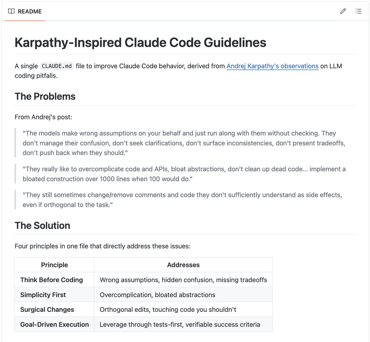
A single 𝗖𝗟𝗔𝗨𝗗𝗘.𝗺𝗱 file just hit 192k GitHub stars.

(derived from Karpathy's coding rules)

Andrej Karpathy observed that LLMs make the same predictable mistakes when writing code: over-engineering, ignoring existing patterns, and adding dependencies you never asked for.

If you've used AI coding assistants, you've hit all of these.

But here's the thing:

If the mistakes are predictable, you can prevent them with the right instructions.

That's exactly what this 𝗖𝗟𝗔𝗨𝗗𝗘.𝗺𝗱 does. You drop one markdown file into your repo, and it gives Claude Code a structured set of behavioral guidelines for your entire project.

This is a big deal.

- Built entirely around prompt engineering for AI coding assistants
- No framework, no complex tooling, just one .md file that shapes behavior

Developers are moving past "use AI to write code" and into "engineer the AI's behavior so the code is actually good."

The Claude Code ecosystem is growing fast, and the best tools in it aren't always software. Sometimes they're just well-crafted instructions.

100% open-source.

Link to the GitHub repo: https://t.co/pq6g88tNE3

That said, I wrote an article on the anatomy of the .claude folder, which was read by 11 million people.

It's a complete guide to 𝗖𝗟𝗔𝗨𝗗𝗘.𝗺𝗱, hooks, skills, agents, and permissions, and how to set them up properly.

The article is quoted below.

[Akshay 🚀 @akshay_pachaar]

the four types of agent loops.

loop engineering keeps getting talked about as one thing. it's actually a choice between four structures, and each one fits a different kind of task.

it means designing the system that steers the agent, instead of steering it yourself move by move.

that system always answers two questions. what starts a run, and what decides the work is done.

in a hand-run session you answer both yourself, every single time. each loop type moves more of that into the system.

here's each type, what triggers it, and when to reach for it.

1) turn-based.

triggered by a user prompt. the agent gathers context, acts, and checks its work inside a single turn, then a human reviews the output and writes the next prompt.

use this when requirements are still forming and every output changes what you'd ask for next.

2) goal-based.

triggered by a /goal command carrying success criteria and a budget, like "get the homepage Lighthouse score to 90, stop after 5 tries." when the agent tries to stop, an evaluator model checks whether the goal is met, and a no sends it back to work.

use this when the outcome is measurable but the path there isn't worth your attention.

3) time-based.

triggered by a clock. an interval fires, the agent runs a fixed prompt like "check the PR, fix CI," then waits for the next tick. /loop runs on your machine, /schedule moves it to the cloud so it survives a closed laptop.

use this for recurring work where the task is known in advance and only the timing repeats.

4) proactive.

triggered by an event or schedule with no human present. a routine watches a channel, and when something needs handling it spawns a workflow with a triage agent, a fix agent, and a reviewer that adversarially judges the work before the task closes.

use this for standing responsibilities where you can't predict what will come in, only that something will.

each type hands off one more job than the last. turn-based keeps both with the human, goal-based automates the checking, time-based automates the trigger, and proactive automates both while deciding the workflow shape at runtime.

so the mapping question isn't which loop is most advanced. it's whether your task is exploratory, measurable, recurring, or standing.

the more you hand off, the less you babysit.

I wrote the full breakdown on loop engineering. the article is quoted below.