Gauthier Dongo

Expert comptable agréé, Sous-directeur à Cpcc | actuellement Associé Gérant de la firme d’audit COREX sarl| Certifié IFRS, Audit des systèmes d’information.

[Excel Easy @ExcelEasy]

Lost in the spreadsheet? Look it up. 🔎 Lookup & Reference Functions in Excel. https://t.co/BN4P86qhzp

[Excel Easy @ExcelEasy]

A, B, C… but smarter. Alphabetize in Excel. https://t.co/qzJ8xnai0C

[Excel Easy @ExcelEasy]

Errors in the range? Ignore them. AGGREGATE function in Excel. https://t.co/SxKjSFARcH

[Tracy Ntumba B.L @Tracy_Ntumba]

❤️

[Excel Easy @ExcelEasy]

Blank cells? Out you go. Delete Blank Cells in Excel VBA. https://t.co/q47sy9onnO

[Excel Easy @ExcelEasy]

Learn how to use Excel. 100% free. Excel Easy for you and me.. and everybody else! 😉 https://t.co/EZ1ULbk8nI

[Excel Easy @ExcelEasy]

One variable? How about five? Array in Excel VBA. https://t.co/2IcXQB7ale

[Excel Easy @ExcelEasy]

What’s that future money worth today? NPV formula in Excel. https://t.co/00w3zGGAQk

[عبدالله @_ABD97]

قام جندي تركي بتربية فتاة كورية تبلغ من العمر 5 سنوات خلال الحـ.رب وبعد 65 عاماً التقيا اخيراً 💔🥹

في عام 1950، ذهب الجندي التركي سليمان ديلبيرليغي إلى كوريا للمشاركة في الحرب الكورية. وهناك وجد طفلة كورية صغيرة وحيدة في وسط الحرب والخراب بعد أن فقدت عائلتها.

أخذها معه واعتنى بها كأنها ابنته، وأطلق عليها اسم «أيلا»، وكانت تناديه «أبي». ❤️

لكن عندما انتهت خدمته، أُجبر على العودة إلى تركيا ولم يستطع أخذ أيلا معه، فتركها في دار للأيتام على أمل أن يلتقيا من جديد.

مرت 60 عاماً تقريباً، قبل أن يجمعهما القدر مرة أخرى… وكانت لحظة اللقاء مؤثرة بشكل لا يُنسى. ❤️

قصة حقيقية تثبت أن بعض الروابط أقوى من الدم، وأن الإنسان قد يترك أثراً في قلب شخص لا ينساه العمر كله. 🥹❤️

[Yoga & Mobility Exercies @YogaMobilitys]

5 hip mobility moves to add to your next warm-up 🔓

Because training isn’t just about what you can do today—it’s about keeping your body moving well for the long run.

[Excel Easy @ExcelEasy]

Money math gets serious. Financial Functions in Excel. https://t.co/qoJ3CYSBiM

[Excel Easy @ExcelEasy]

Just need part of the text? Substring in Excel. https://t.co/HFBoBENxzR

[Aditya Kalyan | Data Analyst 🇮🇳 @ADITYAK37929458]

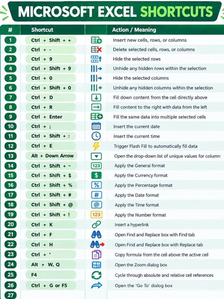
🤯 Excel wizards, this one's for you

🧙‍♀️ Boost your productivity with these game - changing Microsoft Excel shortcuts.

Say goodbye to endless clicking and hello to efficiency.🤩

From inserting rows to applying formats, these tips will transform your workflow.

[Python Programming @PythonPr]

3 Types of machine Learning

[Béatrice Shako (Bs) @Shako_Beatrice2]

Attaque armée à Lubumbashi : le président de la Cour d’appel du Haut-Katanga tué à son domicile.
Le suspect sur la photo.

[Excel Easy @ExcelEasy]

One workbook. Plenty of room. Worksheets in Excel. https://t.co/7Ob2HbWGJV

[Excel Tips & Tricks @exceltipstrick]

How to create a compact table view in Excel 📐

[Tips Excel | AI Productivity @gudanglifehack]

📊 Excel Formulas — Part 4

This part focuses on Lookup formulas — essential when you need to find information from another table.

1️⃣ XLOOKUP

Searches for a value and returns the corresponding result.

=XLOOKUP(A2,E2:E10,F2:F10,"Not Found")

Example: Find an employee's department using their Employee ID.

Why it's useful:

• Can look left or right

• Exact match by default

• Can return a custom result when nothing is found

2️⃣ VLOOKUP

Searches vertically in the first column of a table.

=VLOOKUP(A2,E2:G10,3,FALSE)

Example: Find a product's price using its Product ID.

Remember: FALSE → Exact match

TRUE → Approximate match

3️⃣ HLOOKUP

Searches horizontally across the first row of a table.

=HLOOKUP(B1,B2:F5,4,FALSE)

Useful when your lookup values are arranged horizontally.

4️⃣ INDEX

Returns a value from a specific position in a range.

=INDEX(B2:B10,4)

Example: Return the 4th value from the range B2:B10.

5️⃣ MATCH

Finds the position of a value within a range.

=MATCH("Laptop",A2:A10,0)

0 means you want an exact match.

6️⃣ INDEX + MATCH

A powerful combination for lookups.

=INDEX(C2:C10,MATCH(A2,A2:A10,0))

Here:

MATCH → Finds the position

INDEX → Returns the value from that position

💡 Sample Data

Product ID Product Price

P101 Laptop 50000

P102 Mouse 800

P103 Keyboard 1500

P104 Monitor 12000

P105 Headphones 2500

Try finding the Price for Product ID P103 using:

1. XLOOKUP

2. VLOOKUP

3. INDEX + MATCH

🧠 Double Tap ❤️ For More

[Aditya Kalyan | Data Analyst 🇮🇳 @ADITYAK37929458]

💰 ₹0 Data Analytics Learning Plan.

📊 Excel → @YouTube
🗄️ SQL → @SQLBolt
📈 Power BI → @MicrosoftLearn
🐍 Python → @kaggle
📐 Stats → @khanacademy
📂 Projects → @KaggleDatasets
💻 Portfolio → @github
🔗 Network → @LinkedIn

Just consistency. 🚀

#DataAnalytics #Sql