Just uploaded my "Coding Attention Mechanisms" tutorial. A 2h15m session on coding attention mechanisms to understand how the engine of LLMs works:
self-attention → parameterized self-attention → causal self-attention → multi-head self-attention
https://t.co/bhYtV2cVzv
Maybe a hot take, but what about the following advice to the next gen:
Don't get an AI degree; the curriculum will be outdated before you graduate. Instead, study math, stats, or physics as your foundation, and stay current with AI through code-focused books, blogs, and papers.
I want to show you a clever trick you didn't know before.
Imagine you have six months' worth of data. You want to build a model, so you take the first five months to train it. Then, you use the last month to test it.
This is a common approach for building machine learning models.
Unfortunately, you may find out your model works well with the train data but sucks on the test data.
Overfitting is not weird. We've all been there. But often, the worst you can do is try and fix it before understanding why it’s happening.
Ask anyone about this, and they will give you their favorite step-by-step guide on regularizing a model. They will jump right in and try to fix overfitting. Don’t do this.
There's a different way. A better way.
Here is the question I want you to answer before you start racking your brain trying to fix a model:
Do your test and training data come from the same distribution?
When building a model, we assume the train and test come from the same place. Unfortunately, this is not always the case.
Here is where the trick I promised comes in:
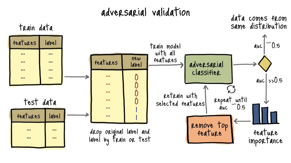
1. Put your train and test set together.
2. Get rid of the target column.
3. Create a new binary feature, and set every sample from your train set to 0 and every sample from the test set to 1. This feature will be the new target.
Now, train a simple binary classification model on this new dataset. The goal of this model is to predict whether a sample comes from the train or the test split.
The intuition behind this idea is simple:
If all your data comes from the same distribution, this model won't work. But if the data comes from different distributions, the model will learn to separate it.
After you build a model, you can use the ROC-AUC to evaluate it. If the AUC is close to 0.5, your model can't separate the samples. This means your training and test data come from the same distribution. If the AUC is closer to 1.0, your model learned to differentiate the samples. Your training and test data come from different distributions.
This technique is called Adversarial Validation. It's a clever, fast way to determine whether two datasets come from the same source.
If your splits come from different distributions, you won't get anywhere. You can't out-train bad data.
But there's more!
You can also use Adversarial Validation to identify where the problem is coming from:
1. Compute the importance of each feature.
2. Remove the most important one from the data.
3. Rebuild the adversarial model.
4. Recompute the ROC-AUC again.
You can repeat this process until the ROC-AUC is close to 0.5 and the model can’t differentiate between training and test samples.
Adversarial Validation is especially useful in production applications to identify distribution shifts.
Low investment with a high return.
The Top ML Papers of the Week (March 4 - March 10):
• Claude 3
• KnowAgent
• LLM for Law
• Design2Code
• RAG Enhancements Overview
• Robust Evaluation of Reasoning
...
The Top ML Papers of the Week (Feb 19 - Feb 25):
- LoRA+
- Gemma
- Stable Diffusion 3
- OpenCodeInterpreter
- Revisiting REINFORCE in RLHF
- CoT Reasoning without Prompting
...
Causal Machine Learning is a new algorithm that combines enhanced causal relationship detection and explainability. Let's dig in.
In today's data-driven landscape, the ability to make accurate predictions and understand the underlying mechanisms of these predictions is invaluable.
Causal ML provides this insight, allowing for more effective decision-making across various domains, from healthcare and economics to marketing and business.
By understanding causality, we can predict the consequences of actions, plan more effective strategies, and avoid unintended outcomes.
At its core, Causal ML seeks to answer "what if" questions: What if a new policy is implemented? What if we change a product's price?
To address these, Causal ML employs various models and tools, such as:
1. Counterfactual Reasoning: Understanding what would have happened under different circumstances.
2. Propensity Score Matching: Comparing groups in observational data as if they were part of a randomized experiment.
3. Causal Inference Techniques: Techniques like Directed Acyclic Graphs (DAGs) and Structural Equation Modeling help identify causal relationships.
===
Want to learn Causal Inference for Data Science?
I have a free workshop, Causal Inference for Data Scientists, Today at 2PM EST.
Inside I'll share my top 3 causal inference techniques (with code) that you can apply to your (future) company's data science projects.
👉 Register Here: https://t.co/wRWLgG5J2I
Log odds. Here’s everything you need to know.
1. The logit function is crucial in machine learning for classification problems. It helps in understanding and predicting categorical outcomes (like yes/no, win/lose).
2. Log odds, also known as the logit function, is a concept used in statistics, especially in logistic regression.
It is the logarithm of the odds ratio, which is the ratio of the probability of an event occurring to the probability of it not occurring.
3. The output of the logit function can be interpreted as the log odds.
For example, a logit value of 0 implies that the odds of the event are even (the event is as likely to occur as not to occur).
Positive logit values indicate higher probability of occurrence, and negative values indicate lower probability.
4. Examples of its application include predicting whether a customer will buy a product, whether a loan will default, and in medical fields for predicting the probability of a disease occurrence based on certain symptoms or test results.
5. The inverse of the logit function is known as the logistic function. It is used to convert log odds back into a probability.
6. It’s essential in logistic regression, a widely used statistical method to model binary outcomes (like yes/no, pass/fail). This has applications in various sectors, from predicting customer behavior to determining the effectiveness of a medical treatment.
=====
Ready to learn more about Data Science, Machine Learning and Business?
I have a free 40-minute webinar where I cover the top 10 skills that helped me on my journey.
👉Learn more here: https://t.co/LR39RJ5XKB
Ordinary Least Squares (OLS) Regression is one of the most important tools in a Data Scientist's toolbox. Here's everything you need to know.
1. OLS regression aims to find the best-fitting linear equation that describes the relationship between the dependent variable (often denoted as Y) and independent variables (denoted as X1, X2, ..., Xn).
2. OLS does this by minimizing the sum of the squares of the differences between the observed dependent variable values and those predicted by the linear model. These differences are called "residuals."
3. "Best fit" in the context of OLS means that the sum of the squares of the residuals is as small as possible. Mathematically, it's about finding the values of β0, β1, ..., βn that minimize this sum.
4. Slopes (β1, β2, ..., βn): These coefficients represent the change in the dependent variable for a one-unit change in the corresponding independent variable, holding other variables constant.
5. R-squared (R²): This statistic measures the proportion of variance in the dependent variable that is predictable from the independent variables. It ranges from 0 to 1, with higher values indicating a better fit of the model to the data.
6. t-Statistics and p-Values: For each coefficient, the t-statistic and its associated p-value test the null hypothesis that the coefficient is equal to zero (no effect). A small p-value (< 0.05) suggests that you can reject the null hypothesis.
7. Confidence Intervals: These intervals provide a range of plausible values for each coefficient (usually at the 95% confidence level).
Understanding and interpreting these outputs is crucial for assessing the quality of the model, understanding the relationships between variables, and making predictions or conclusions based on the model.
====
Ready to learn Data Science for Business?
I put together a free on-demand workshop that covers the 10 skills that helped me make the transition to Data Scientist: https://t.co/LR39RJ5XKB
And if you'd like to speed it up, I have a live workshop next week where I'll share how to use ChatGPT for Data Science: https://t.co/EaMpKrJiqX
Logistic Regression is the most important foundational algorithm in Classification Modeling. In 2 minutes, I'll teach you what took me 2 months to learn. Let's dive in:
1. Logistic regression is a statistical method used for analyzing a dataset in which there are one or more independent variables that determine a binary outcome (in which there are only two possible outcomes). This is commonly called a binary classification problem.
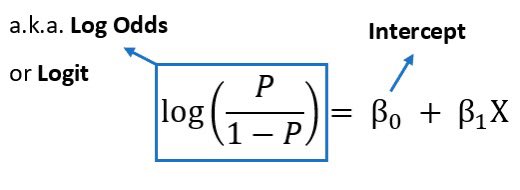
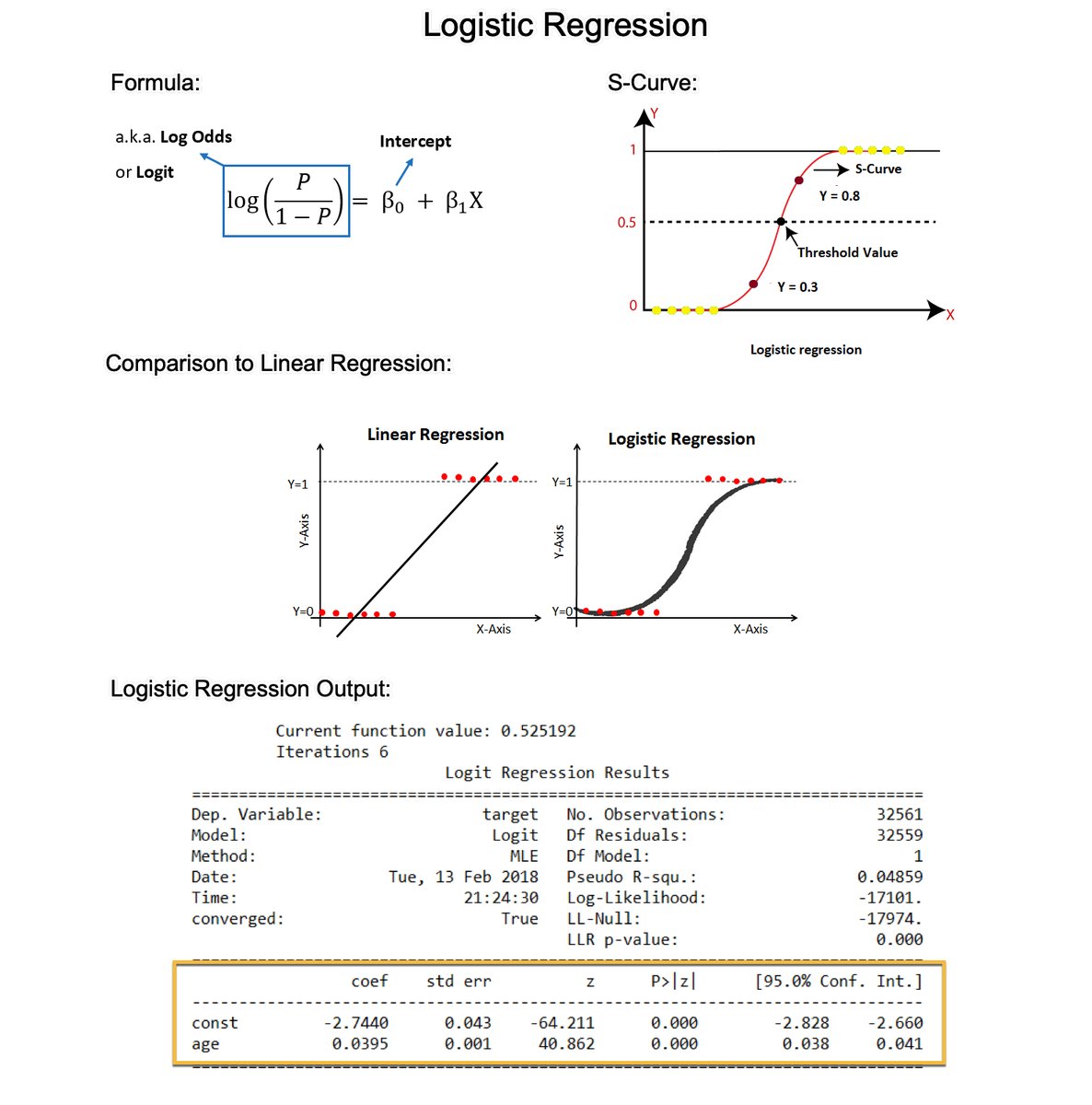
2. The Logit (Log-Odds): The formula estimates the log-odds or logit. The right-hand side is the same as the form for linear regression. But the left-hand side is the logit function, which is the natural log of the odds ratio. The logit function is what distinguishes logistic regression from other types of regression.
3. The S-Curve: Logistic regression uses a sigmoid (or logistic) function to model the data. This function maps any real-valued number into a value between 0 and 1, making it suitable for a probability estimation. This is where the S-curve shape comes in.
4. Why not Linear Regression? The shape of the S-curve often fits the binary outcome better than a linear regression. Linear regression assumes the relationship is linear, which often does not hold for binary outcomes, where the relationship between the independent variables and the probability of the outcome is typically not linear but sigmoidal (S-shaped).
5. Coefficient Estimation: Like linear regression, logistic regression calculates coefficients for each independent variable. However, these coefficients are in the log-odds scale.
6. Coefficient Interpretation (Log-Odds to Odds): Exponentiating a coefficient converts it from log odds to odds. For example, if a coefficient is 0.5, the odds ratio is exp(0.5), which is approximately 1.65. This means that with a one-unit increase in the predictor, the odds of the outcome increase by a factor of 1.65.
7. Model evaluation: The evaluation metrics for linear regression (like R-squared) are not suitable for assessing the performance of a model in a classification context. For Logistic regression, I normally use classification-specific evaluation metrics like AUC, precision, recall, F1 score, ROC curve, etc.
===
Ready to learn Data Science for Business?
I put together a free on-demand workshop that covers the 10 skills that helped me make the transition to Data Scientist: https://t.co/LR39RJ5XKB
And if you'd like to speed it up, I have a live workshop next week where I'll share how to use ChatGPT for Data Science: https://t.co/EaMpKrJiqX
Prof. Gilbert Strang gave his final lecture today!
End of an era. His linear algebra lectures where the best of the best 👌.
His lectures are a treasure, and I hope they will remain accessible indefinitely: https://t.co/oLktEaF9Mc
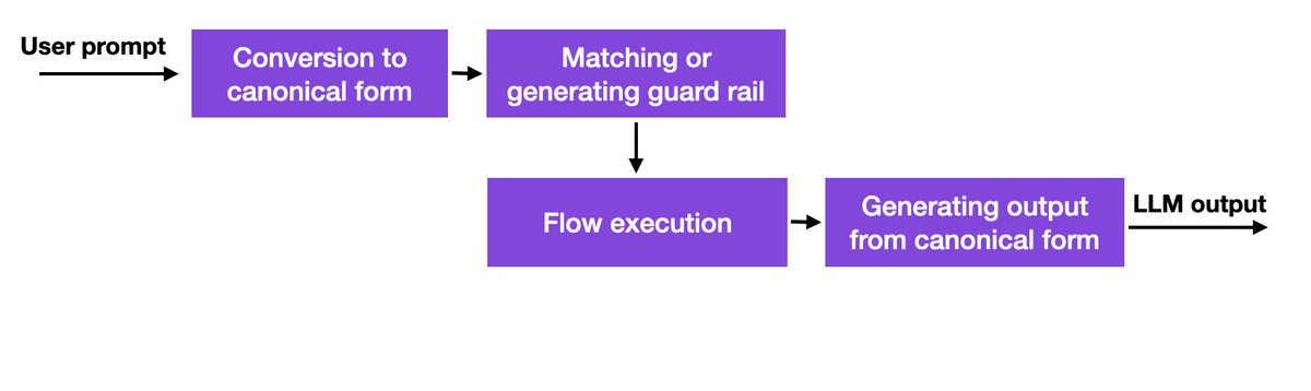
Nvidia open-sourced a toolkit to address the hallucination issue (/capabilities) of LLMs called NeMo Guardrails. In a nutshell, how it works is that this method uses a database linking to hardcoded prompts, which have to be manually curated.
Repo: https://t.co/cvD91D9Ujz
1/4
Hope you all are having a great day 😊
Everywhere news, LinkedIn, YouTube is flooded with laid off posts.
Everyone is showing support to them. And one should be.
This is the worst one can think of. But I wonder how freshers will get into the industry at such a bad time.