B. Noted

Welcome to the B. Noted Network, where data science is remade into a fascinating trip of insightful, bite-sized content with a cartoon twist.

[B. Noted @LetIt_BNoted]

B. Noted is a distinguished data science authority, widely recognized for his substantial contributions to academic research and practical applications. His seventh acclaimed textbook, "Statistical and Machine-Learning Data Mining of Big Data" (3rd edition), has become a bestseller and emerged as an essential reference for students, educators, and professionals seeking to deepen their understanding of complex data analysis. This comprehensive guide thoroughly examines the multifaceted world of data analysis, offering clear, accessible explanations of intricate concepts alongside innovative methodologies that are crucial for effectively navigating the myriad challenges presented by big data. In addition, B. Noted has published 100+ peer-reviewed articles and holds a patent on a genetic programming algorithm that surplants classical regression techniques.

In addition to his impressive academic background, B. Noted has crafted a formidable reputation within the consulting domain, where he expertly applies his extensive knowledge to solve real-world challenges. He collaborates with clients spanning various industries and sectors, each seeking his insights to enhance their marketing decision-making processes. His clients frequently praise his exceptional ability to dissect complex issues, allowing them to make informed choices based on data-driven insights.

B. Noted takes a highly customized and analytical approach to problem-solving, ensuring that his proposed solutions are specifically tailored to each client’s unique circumstances, thus delivering optimal and impactful results. His unwavering commitment to punctuality and excellence further strengthens client relationships, fostering trust, reliability, and long-term collaboration.

Beyond his consulting endeavors,
B. Noted has become a highly sought-after speaker, frequently invited to share his insights at prestigious industry conferences, including the renowned SAS Data Mining Conferences. His participation in exclusive seminars hosted by some of the Fortune Magazine Top 100 Companies highlights his standing in the industry, as he imparts valuable knowledge to influential leaders and professionals.

B. Noted’s expertise is further complemented by his proficiency in programming languages, including SAS, R, and Python. This diverse skill set enables him to tackle a wide array of data-related projects, combining technical acumen with a strategic mindset. He ultimately drives impactful outcomes reflecting his deep understanding of data science's theoretical and practical dimensions. Through his multifaceted pursuits, various contributions continue to leave a profound mark on the field, shaping the future of data analysis and its applications in numerous sectors.


[B. Noted @LetIt_BNoted]

*** Principal Component Analysis: A Practical Overview ***
Principal Component Analysis (PCA) is a dimensionality reduction technique in statistics and machine learning. It transforms high-dimensional data into a lower-dimensional form while preserving as much variance as possible, making complex datasets easier to analyze, visualize, and process.

The Core Idea
Many features in a dataset are often correlated, carrying overlapping information. PCA identifies the directions in which the data varies the most and projects the data onto those directions, called principal components, producing a new set of uncorrelated variables that capture the essential structure of the original data.

How PCA Works
First, each feature is standardized to have a mean of 0 and a variance of 1, ensuring no single feature dominates due to scale. Next, the covariance matrix is computed to capture linear relationships between features. This matrix is then decomposed into eigenvectors and eigenvalues, where each eigenvector defines a direction in feature space and its eigenvalue indicates the variance along that direction. The top eigenvectors, those with the largest eigenvalues, become the principal components. Finally, the original data is projected onto these components, producing a reduced-dimensional representation.

Explained Variance
Each principal component accounts for a percentage of the total variance. Practitioners typically retain enough components to explain 90–95% of the variance. A scree plot, graphing eigenvalues against component number, is a common tool for deciding how many components to keep.

Applications
PCA is used across many fields. It speeds up machine learning algorithms by reducing features, enables visualization of high-dimensional data in 2D or 3D, filters noise from datasets, compresses images, reveals population structure in genomics, and identifies risk factors in finance.

Limitations and Extensions
PCA assumes that maximum variance equals maximum information, which does not always hold. It is linear, sensitive to outliers, and produces components that can be difficult to interpret. Extensions such as Kernel PCA handle non-linear relationships, Sparse PCA improves interpretability, and Robust PCA manages outliers more effectively.

Despite being rooted in century-old linear algebra, PCA remains one of the most practical and widely used tools in modern data science.
--- B. Noted


[B. Noted @LetIt_BNoted]

*** Data Science Disasters: Common Ways We Misinterpret and Misuse Data ***
Data science is an incredibly powerful tool, but like any powerful tool, it gets misused all the time. Sometimes it's accidental due to a lack of training, and other times it's a deliberate attempt to make data fit a preferred narrative.
Here is a breakdown of the most common ways data science goes wrong and how to spot them.

P-Hacking and Data Dredging
This happens when researchers or analysts run hundreds of tests on a dataset until they find one that is statistically significant, and then they report only that single result. If you test enough random variables, pure chance dictates that eventually, you will find a pattern that looks meaningful but is actually just noise.
To fix this, hypotheses should be formed before looking at the data, not after.

Mistaking Correlation for Causation
This is the classic data science trap. Just because two data points move together does not mean one caused the other. For example, ice cream sales and shark attacks both spike during the summer. A flawed model might claim buying ice cream causes shark attacks, ignoring the lurking variable: warm weather.
Always look for the underlying mechanism before claiming one thing caused another.

Selection Bias and Survivorship Bias
Your model is only as good as the data you feed it. If your data collection method inherently excludes certain groups, your conclusions will be fundamentally flawed.
A famous example of survivorship bias comes from World War II, where armor was placed on planes. Analysts examined returning bombers to see where they were hit hardest, concluding that those areas needed more armor. But they forgot to account for the planes that didn't return. The planes that crashed were hit in different, vital areas.
If you only analyze the survivors or the easiest data to reach, you miss the full picture.

Overfitting the Model
When building machine learning models, there is a temptation to make the algorithm perfectly match the training data. When this happens, the model memorizes the training data, including its random quirks and errors, rather than learning the general trend.
As a result, the model looks incredibly accurate on paper but fails miserably when introduced to real-world, unseen data. A good model should prioritize simplicity and generalizability over perfection on a single dataset.

The Black Box Problem
With the rise of deep learning, it has become easier to build highly complex models that produce accurate predictions but offer no explanation of how they arrived at those conclusions.
Relying unthinkingly on a black box can be dangerous, especially in high-stakes fields like healthcare, finance, or criminal justice. Without interpretability, it is almost impossible to diagnose when a model is exhibiting bias or failing quietly under the surface.

Ignoring the Baseline
Data can easily be manipulated to look dramatic when it isn't. For instance, a headline might scream that a new habit doubles your risk of a certain disease. That sounds terrifying. However, if the baseline risk of getting that disease were 1 in a million, doubling it would only raise it to 2 in a million.
Always look for the absolute context, not just the relative percentage changes.
--- B. Noted


[B. Noted @LetIt_BNoted]

*** A Data Scientist’s Guide to Using "Myself" Effectively ***
In the world of data science, your ability to communicate complex findings is just as critical as your ability to build models. Whether you are presenting a dashboard to stakeholders or writing documentation for your team, your writing style reflects your professional rigor.

One common area where precision often falters is the usage of the pronoun "myself." According to A Guide to Using Myself, the word is a reflexive or intensive pronoun used in three primary ways.
1. Reflexive Use
This is the most common form, occurring when the subject and the object of a sentence are the same person, meaning the verb "reflects" back onto the person performing it.
Definition: The subject does something to themselves.
Example: "I accidentally cut myself while chopping vegetables".
Example: "I told myself that everything would be okay".

2. Intensive (Emphatic) Use
In this context, "myself" emphasizes the subject. If you remove the word, the sentence remains grammatically correct, and its core meaning does not change.
Definition: Used for emphasis or to indicate that the subject acted without help.
Example: "I myself prefer to walk rather than drive".
Example: "I built the bookshelf myself" (this emphasizes that no one else was involved).

3. Idiomatic or Informal Use
Sometimes, "myself" is used in place of "me" or "I," particularly in compound structures. While strict grammarians may label this as informal or non-standard, it remains very common in casual speech.
As an object in a compound phrase: "They invited my wife and myself to dinner" (though "my wife and me" is preferred in formal grammar).
For self-reference: "I’d like to introduce myself".

Why this matters for your career:
Data science is a collaborative field. When you write clearly and correctly, you reduce ambiguity and build trust with your audience. By mastering nuances like the proper use of "myself," you demonstrate that you pay as much attention to your communication as you do to your data.
--- B. Noted


[B. Noted @LetIt_BNoted]

*** The Erosion of Craft: Why AI is Stunting the Growth of Junior Data Scientists ***
The claim that AI is degrading the skills of junior data scientists is sparking intense debate. As tools integrate into data workflows, concerns grow that we are witnessing an erosion of fundamental analytical capabilities.

The core issue lies in relying on generative AI for coding and problem-solving. When junior data scientists use models to write SQL or Python code, they bypass the cognitive effort required to master these languages. Instead of debugging by analyzing logic, they have the model fix the code. This creates a feedback loop that outsources critical thinking.

This dependency creates a fragile foundation. Data science requires understanding the mechanics of data manipulation, the nuances of statistics, and the limitations of models. When practitioners don’t understand why code works, they cannot troubleshoot when tools fail or provide incorrect answers. They become operators of black-box technology rather than scientists who understand the underlying logic.

Furthermore, automation may stifle the development of professional intuition. Senior practitioners built expertise through trial and error, a slow process that AI accelerates. By receiving instant answers, juniors may miss the chance to hypothesize, test, and fail—a cycle essential for mastery.

Additionally, without the depth to validate AI output, junior scientists may propagate flawed methodologies. Lacking the knowledge to spot subtle errors in architecture or statistics can lead to inaccurate insights.

While AI can act as a force multiplier for experienced professionals, the danger lies in a culture prioritizing speed over mastery. The challenge is ensuring AI supplements, rather than substitutes for, foundational learning. Without prioritizing the theory behind data science, we risk creating a generation of practitioners efficient at prompting but unprepared for the complexities of real-world work.
--- B. Noted


[B. Noted @LetIt_BNoted]

XGBoost stands for eXtreme Gradient Boosting. It is an efficient, flexible machine learning algorithm used for supervised learning tasks such as classification and regression.

Why Boosting Works
Boosting works by combining multiple weak learners, typically simple decision trees, to create a single strong learner. The core idea is iterative improvement. Instead of training models independently, boosting trains them sequentially. Each new model focuses on correcting the errors introduced by combining all previous models. By focusing on hard-to-predict data points that previous trees misclassified or mispredicted, the model gradually reduces total error, resulting in high predictive accuracy.

XGBoost Differs from Random Forest
While both are ensemble methods based on decision trees, they operate differently.

Random Forest uses Bagging. It builds multiple decision trees in parallel, each on a random subset of the training data. The final output is an average or a majority vote of all trees. This approach aims to reduce variance, making the model robust against noise.

XGBoost uses Boosting. It builds shallow trees sequentially. Each tree tries to optimize the objective function using the residuals from previous trees. Because it learns from mistakes, it is generally more accurate than Random Forest but can be more prone to overfitting if not properly tuned. XGBoost also includes built-in regularization and handles missing data natively, whereas Random Forest typically requires pre-processing to handle them.

Bias-Variance Tradeoff
The bias-variance tradeoff is a central concept in model performance.
Bias refers to the error introduced by approximating a complex real-world problem with a simplified model. High bias leads to underfitting, where the model is too simple to capture the underlying patterns in the data.

Variance refers to the error introduced by the model's sensitivity to small fluctuations in the training set. High variance leads to overfitting, where the model captures noise rather than the signal, performing well on the training data but poorly on unseen data.

Boosting aims to reduce bias by incrementally improving the fit to the data. However, as the model becomes more complex with many trees, it risks increasing variance.

Overfitting and Regularization
XGBoost mitigates overfitting by regularization, which penalizes overly complex models.

L1 Regularization (Lasso) and L2 Regularization (Ridge) are integrated directly into the objective function. These penalties discourage large weights in the model, effectively simplifying the decision boundaries created by the trees. Additionally, XGBoost employs techniques such as tree pruning, which removes branches that do not contribute significantly to the predictive power, and subsampling (row and column sampling) during the construction of each tree. These methods ensure the model generalizes well to new data rather than just memorizing the training set.
--- B. Noted


[B. Noted @LetIt_BNoted]

*** Generalized Linear Models: The Power and Flexibility of GLMs ***
Generalized Linear Models (GLMs) are a powerful class of statistical models that extend the traditional linear regression framework. They are widely used because they allow us to predict a response variable that doesn't necessarily follow a normal distribution, making them incredibly flexible for real-world data analysis.

The Core Idea
In a standard linear regression, we assume that the relationship between our predictor variables and the outcome is a straight line and that the errors are normally distributed. However, many real-world outcomes do not fit this mold. For example, if you are predicting whether a customer will buy a product (yes/no) or counting how many website visits occur in an hour (0, 1, 2, 3...), standard linear regression falls short because it can predict impossible values, like negative counts or probabilities above 100 percent.

GLMs solve this by introducing three key components:
1. The Random Component: This specifies the conditional distribution of the response variable. Instead of being restricted to a normal distribution, it can belong to any distribution within the exponential family, which includes the Normal, Binomial, Poisson, Gamma, and Inverse Gaussian distributions.
2. The Systematic Component: This is the linear combination of the predictor variables, often called the linear predictor. It represents the structural part of the model that explains the data's variation.
3. The Link Function: This is the magic ingredient of a GLM. The link function is a mathematical function that connects the linear predictor to the expected value of the response variable. It ensures that the model's predictions remain within valid, realistic bounds.

Common Types of GLMs
Depending on the nature of your data, you will choose a specific distribution and its corresponding link function.
Linear Regression: This is actually just a special case of a GLM where the random component is normally distributed, and the link function is the identity function, meaning it does not alter the relationship.
Logistic Regression: Used when the outcome is binary, such as predicting whether a patient has a disease or not. It uses a binomial distribution and a logit link function, which constrains the final predictions to be strictly between 0 and 1.
Poisson Regression: Used for count data, like the number of insurance claims made in a year. It uses a Poisson distribution and a log link function, ensuring that predicted counts are always greater than or equal to zero.

Why GLMs are Preferred
GLMs provide a unified framework for modeling diverse data types without requiring complex data transformations. By choosing the right distribution and link function, researchers and data scientists can build robust models that accurately reflect the underlying physical or behavioral processes they are trying to understand.
--- B. Noted


[B. Noted @LetIt_BNoted]

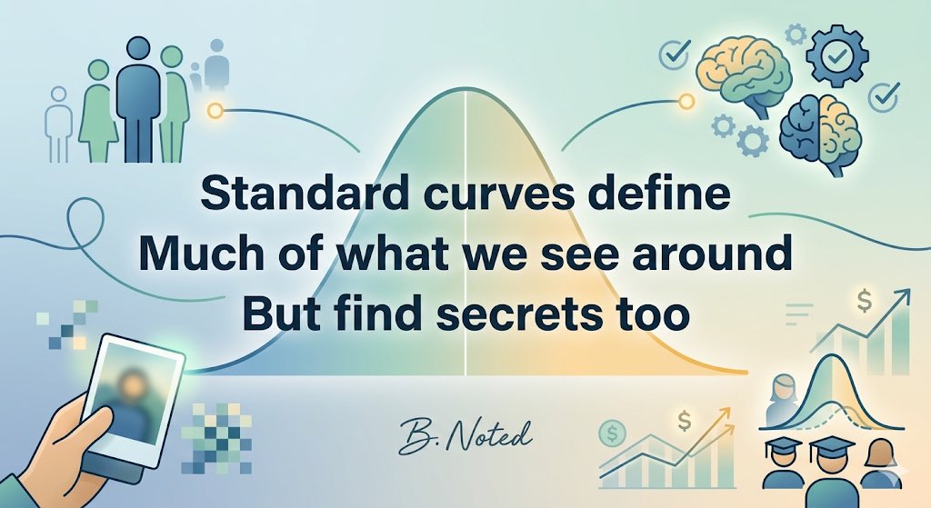
*** 3 Unexpected Uses of the Normal Distribution ***
The normal distribution, often called the bell curve, is famous for describing everyday data like human heights, IQ scores, or test results. However, its mathematical properties allow it to solve some surprisingly weird, creative, and critical problems across different industries.
Here is how the normal distribution is used in unique and unexpected ways.

The Beer and Soda Dilemma: Minimizing "Overfill"
If a beverage company sells a 12-ounce can of soda, every single can must contain at least 12 ounces to comply with consumer protection laws. However, liquid-filling machines aren't perfect; the amount they dispense varies slightly from can to can, forming a normal distribution.
To ensure almost zero cans fall below the 12-ounce mark, factories don't set the machine to pour exactly 12 ounces. Instead, they use the machine's standard deviation of pours to calculate an average filling target slightly above 12 ounces—say, 12.1 ounces. By understanding the exact shape of the bell curve, companies can calculate the precise economic sweet spot: protecting themselves from legal trouble while saving millions of dollars a year by avoiding overfilling.

The Netflix and Spotify Secret: Standardizing Human Chaos
When you rate a movie on a scale of 1 to 5, your "4" might mean "I loved it," while a harsher critic's "4" might mean "It was just okay." Human behavior and rating habits are notoriously messy and inconsistent.
To fix this, recommendation algorithms use the normal distribution to normalize user data. They transform a user's raw ratings so that the user's personal average becomes the center of a standard normal distribution. By converting raw scores into "standard scores" (z-scores), the algorithm can accurately compare a harsh critic to an easy grader, ultimately predicting what you want to watch next.

Setting the Price of Financial Risk: The Black-Scholes Model
In the stock market, predicting a stock's exact future price is impossible. However, financial theorists realized that while stock prices themselves don't follow a normal distribution, the log-returns (the percentage changes in price over tiny time increments) do.
This insight forms the foundation of the Black-Scholes model, a Nobel Prize-winning formula used to price financial options. By treating market volatility as a normal distribution, Wall Street can calculate the probability that a stock will hit a given price by a given date. This allows investors to put a fair price tag on financial risk.
--- B. Noted


[B. Noted @LetIt_BNoted]

*** Equally Likely: Understanding the Uniform Distribution ***
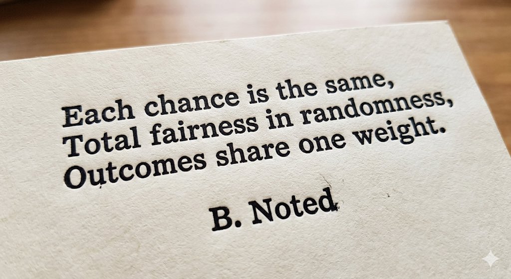
Imagine a perfectly fair, traditional six-sided die. When you roll it, the chance of landing on a 1 is the same as landing on a 2, a 3, a 4, a 5, or a 6. No single number has an advantage over the others.
This is the core concept of a Uniform Distribution. It is a type of probability distribution in which every possible outcome has an equal probability of occurring. In the world of statistics, it represents ultimate fairness and predictability in terms of likelihood, even though the individual outcomes themselves are random.

There are two main types of uniform distributions, depending on what you are measuring.
The first is the Discrete Uniform Distribution. This applies to situations where you can count the possible outcomes on your fingers, like rolling a die, flipping a coin, or drawing a specific card from a well-shuffled deck. The outcomes are distinct, separate points, and each one holds an identical slice of the probability pie.

The second is the Continuous Uniform Distribution. This applies to scenarios where the outcomes can be any value within a certain range, including fractions and decimals.
To picture this, imagine you are waiting for a bus that arrives strictly every thirty minutes, but you have no idea what time it actually is when you walk up to the bus stop. Your waiting time could be 2 minutes, 15 minutes, or 29 minutes and 59 seconds. Every single exact moment within that thirty-minute window is equally likely.

When you look at a visual graph of a continuous uniform distribution, it looks like a flat, solid rectangle. The bottom of the rectangle spans the minimum and maximum possible values. The rectangle's height remains perfectly level across the top. This flat line represents the constant, unchanging probability across the entire range. Because the total probability of any event must always equal one hundred percent, the area inside this rectangle always represents certainty, and you can find the likelihood of an event by looking at the width of the section you are interested in.

In the real world, uniform distributions are incredibly useful, especially in technology and simulations.
For instance, whenever a video game generates a random map or a computer selects a random winner for a sweepstakes, it relies on a random number generator. These software tools are designed around a uniform distribution to ensure that every user or every possible number has an equal chance of being selected, preventing bias.
It is also used as a baseline in data science when researchers have absolutely no prior knowledge about a situation. If you have no reason to believe one outcome is more likely than another, assuming a uniform distribution is the most honest and unbiased starting point.
--- B. Noted


[B. Noted @LetIt_BNoted]

*** Optimizing the Soul: The Bamboo Strategy of Data Science ***
Here is an interpretation of the famous Chinese proverb—“A bamboo branch bends, but does not break” (竹子能弯也能伸)—tailored for a data scientist, translating the concept of resilience, flexibility, and architectural strength into the language of system design and training:
"The distribution shifts, bending the architecture to its limit,
Yet an elastic regularization yields without breaking,
Restoring equilibrium to the shifting pipeline."

The Breakdown
“A bamboo branch bends...”
▶️ Data Drift / Distribution Shift: Represents the sudden, harsh pressure external reality puts on a static deployment. The incoming production data changes, threatening to render the features obsolete and destabilize accuracy.
“...but does not break...”
▶️ Elastic Net / Dynamic Thresholding: The built-in mathematical flexibility (combining L1 and L2 regularizers) that allows the parameters to absorb the shock. Instead of exploding or returning null values, the weights adjust dynamically to accommodate the new strain.
“...yields without breaking.”
▶️ Self-Healing Pipeline / Model Robustness: The ultimate triumph of flexible engineering. The architecture absorbs the edge cases, gracefully handles the anomalies, and maintains system uptime through pure structural adaptability.
--- B. Noted


[B. Noted @LetIt_BNoted]

*** Stop Using OLS for Percentages and Proportions ***
Ever tried using standard linear regression (OLS) on percentages, only to have your model predict a revenue share of 115%?
If you're modeling dependent variables that live strictly between 0 and 1—like market shares, recovery rates, or budget allocations—traditional OLS breaks down.

Enter the Fractional Logit Model.
Here is why this powerhouse model belongs in your data science toolkit, and why it beats standard regression for proportion data:

The Problem with OLS for Proportions
When your data is bounded between 0 and 1, Ordinary Least Squares throws a tantrum:
Boundary Violations: It can easily produce nonsense values such as -0.2 or 1.3.
Heteroscedasticity: Variance inherently shrinks near the 0 and 1 boundaries, violating OLS assumptions.
Non-Normality: Proportion data is rarely normally distributed.

The Fractional Logit Fix
Instead of forcing a straight line onto a bounded problem, the Fractional Logit model uses a quasi-maximum likelihood estimation (QMLE) approach with a logit link function.
Mathematically, it models the conditional mean as:
E(Y|X) = exp(Xb) / (1 + exp(Xb))
This elegant math ensures your predictions always remain within the [0, 1] interval.

Key Execution & Interpretation Tips
1. Estimation: You don't need exotic software. Any GLM framework (like statsmodels in Python or glm in R) using a logit link and the binomial family will do the heavy lifting.
2. Interpretation: Raw coefficients (beta) represent log-odds, which can be tough to explain to stakeholders. Pro-tip: Always compute Marginal Effects to show the actual change in percentage points for a one-unit change in your predictor.

The Trade-Off
The Good: It’s incredibly robust, handles non-normality seamlessly, and respects the boundaries of your data.

The Catch: It requires a bit more computational juice and a layer of translation for non-technical audiences compared to a simple linear trend.

The Bottom Line: If your data lives in fractions, stop forcing it into linear boxes. Fractional logit models offer the exact mathematical guardrails your analysis needs.
--- B. Noted


[B. Noted @LetIt_BNoted]

*** The OLS Trap: Why Your Linear Model Might Be Precise, But Totally Untestable ***
Ordinary Least Squares (OLS) regression is the "gold standard" for data modeling. If you’ve studied probability or data science, you know its ultimate prize: achieving BLUE (Best Linear Unbiased Estimator) status.
But there is a massive trap that catches data professionals off guard: The distinct line between making a model efficient and making it testable.

Here is the breakdown of the 5 vs. 6 Assumptions framework, and why the difference matters for your deployment.
⚖️ 1. The Core Distinction: Efficiency vs. Inference
Think of these two frameworks as different "service tiers" for your data:
The Gauss-Markov Theorem (5 Assumptions) = The Efficiency Guarantee
The Goal: Prove that OLS is the most precise way to estimate coefficients.
The Output: You achieve BLUE status. Your coefficients are unbiased and have the minimum possible variance.
The Full OLS Tier (6 Assumptions) = The Inference Package
The Goal: Allow for actual prediction and hypothesis testing.
The Output: You can suddenly trust your p-values, t-stats, and confidence intervals to prove statistical significance.

🎯 2. The Dealbreaker: Normality
What is the actual difference between the 5-assumption and 6-assumption models? The Normality of Residuals.
Gauss-Markov doesn't care about normality. As long as the errors have a mean of zero and constant variance (homoscedasticity), your coefficients are optimized.
Full OLS demands normality. Without a bell-curve distribution of errors, traditional t-tests and p-values completely break down—even if your coefficients are technically accurate.
⚠️ The Takeaway: You can have the most mathematically precise line of best fit (by minimizing your Sum of Squared Errors), but without that 6th assumption, you cannot statistically prove why it fits.

🧠 The Quick Summary
5 Assumptions (Gauss-Markov): Makes your model efficient ("My coefficients are precise.")
6 Assumptions (Full OLS): Makes your model testable ("I can actually trust my p-values.")

Before you ship your next model, ask yourself: Are you just trying to fit a line, or are you trying to prove a hypothesis?
--- B. Noted


[B. Noted @LetIt_BNoted]

*** The Linear Regression Trap: Curvature, Multicollinearity, and Higher Dimensions ***
Most people think Ordinary Least Squares (OLS) can only draw straight lines.
They are wrong.
"Linear" means linear in the weights (beta), not the features (X). This means you can model intense, sweeping curves inside a standard linear regression simply by adding polynomial terms (X^2, X^3).

To OLS, a squared feature is just another variable. It solves it instantly.
But this flexibility hides a massive statistical trap. 💥
🪤 The Trap: Runaway Variance
Adding higher-order terms (X, X^2, X^3) introduces severe multicollinearity. Because these features are built from the same data, they move tightly together.
This makes your calculation matrix mathematically fragile and unstable.

The consequences?
Exploding Variance: Your margins of error for your multipliers skyrocket.
Extreme Instability: Tiny tweaks to your training data cause massive, erratic weight shifts.
The "Wiggle" Phenomenon: The model masterfully hits your training points, but oscillates wildly between them (overfitting).

🛠️ The Fix: Stabilize Your Matrix
You don't need to abandon OLS for a complex machine learning algorithm. You need to transform your data before fitting it:
1. Mean Centering: Subtracting the average from your original feature instantly breaks down the correlation between the standard and higher-order terms.
2. Orthogonal Polynomials: A more robust transformation that ensures every single curved term is completely uncorrelated, keeping your matrix rock-solid.
💡 The Big Takeaway
Don't judge a model by its plot geometry; look at its structural framework.
If the weights stand alone, OLS can handle it.
Complex curves are often just straight lines masquerading in a higher dimension.
--- B. Noted


[B. Noted @LetIt_BNoted]

*** Bridging Statistical Intuition and Explicit Logic in Next-Generation AI ***
The artificial intelligence industry is undergoing a significant transition from the previously held belief that scale alone could facilitate reasoning to an acknowledgment of the limitations inherent in monolithic Large Language Models (LLMs) when addressing complex logical tasks.

Although larger models enhance fluency, they continue to encounter systematic deficiencies, such as mathematical inaccuracies and fragile causal sequences.

This evolution has fostered a shift towards 'system orchestration,' wherein AI systems collaborate with specialized tools, alongside the emergence of Neuro-symbolic AI that integrates neural perception with explicit logical frameworks.

Philosophical discourse persists regarding whether the human brain is fundamentally Bayesian; however, current AI systems do not possess true belief systems. Ultimately, future advancements in AI are expected to blend statistical intuition with formal logic, surpassing mere word prediction capabilities.
--- B. Noted


[B. Noted @LetIt_BNoted]

*** Beyond the Reach of Proof: What Gödel's Theorem Actually Means ***
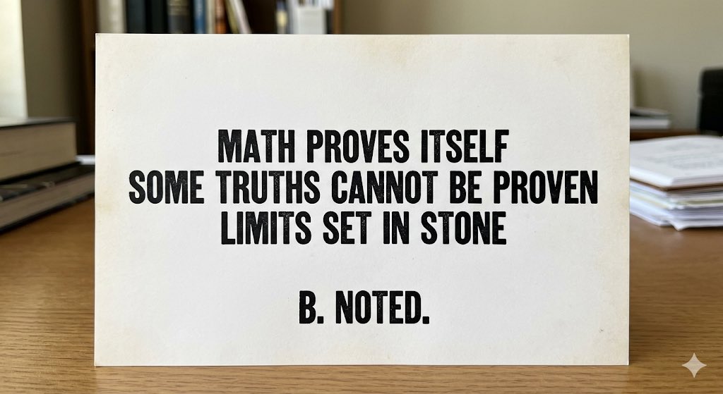
Kurt Gödel's Incompleteness Theorem is often treated as mystical philosophy, but it is actually a precise mathematical proof of the limits of mathematical systems.

In the early 20th century, mathematicians wanted to build a perfect, rock-solid foundation for all of mathematics. They wanted a system of basic assumptions (called axioms) that could prove every true mathematical statement, and never prove anything false.
Gödel proved that this perfect system is mathematically impossible.
The core of his discovery boils down to two main rules that apply to any consistent mathematical system capable of doing basic arithmetic:
1. The system can never be both complete and consistent. If the system is consistent (meaning it contains no contradictions), there will always be true statements within that system that cannot be proven using its own rules.

2. The system cannot prove its own consistency. You cannot use the rules of the system to prove that the system itself will never lead to a contradiction.
To achieve this, Gödel used a brilliant trick now known as Gödel Numbering. He assigned a unique number to every mathematical symbol, variable, and equation. By doing this, he allowed mathematics to look at itself and talk about itself.
Using this code, he constructed a specific mathematical statement that essentially says: "This statement cannot be proven using the rules of this system."
If the system *can* prove that statement, then the statement is false, which means the system is inconsistent and broken. If the system *cannot* prove it, then the statement is true, which means the system is incomplete.

Ultimately, Gödel's Theorem is about intellectual humility in the face of logic. It shows us that truth is a larger concept than proof. No matter how powerful or comprehensive we make our logical systems, there will always be truths that lie just beyond the reach of our formal rules.
--- B. Noted


[B. Noted @LetIt_BNoted]

*** The Linear Regression Trap: Linearity in the Parameters ***
When introductory textbooks list the assumptions of Ordinary Least Squares (OLS) regression, they almost always list the first assumption simply as: Linearity.
This single word is a pedagogical trap. It causes students to look at a curved scatterplot and incorrectly conclude, "We can't use linear regression here."
But you can. OLS does not care if the data points form a straight line. It only requires Linearity in the Parameters.

The Two Types of Linearity
To clear up the confusion, we have to separate the data from the weights (beta coefficients):
Line-1: Linearity in the Variables: The relationship between y and x must look like a straight line on a graph.
Line-2: Linearity in the Parameters: The unknown weights (beta) must enter the equation as a simple sum of products. They cannot be squared, divided, or used as exponents.
OLS completely ignores the first type and strictly demands the second.

The Comparison
Here is how to instantly spot the difference when looking at a model's equation:
```
[MODEL A] y = β₀ + β₁x + β₂x² + ε --> VALID FOR OLS

```
Why it works: Look at the data (x). It is squared, which means the graph will be a curve (a parabola). But look at the parameters (beta). Each beta is just sitting there naturally, waiting to be multiplied. Because the parameters are linear, OLS handles this curved relationship with ease.
```
[MODEL B] y = β₀ + (x / (β₁ + x)) + ε --> INVALID FOR OLS

```
Why it fails: Here, beta1 is trapped in the denominator. You cannot separate it using standard linear-algebra matrices. This is truly non-linear, requiring specialized non-linear estimation techniques.

The Takeaway: Data can bend, twist, and curve. As long as your parameters are standing in a straight line, you are doing linear regression.
--- B. Noted



[B. Noted @LetIt_BNoted]

*** Life in a World Without e ***
What would intellectual life look like if we had to live without the mathematical constant e? Named after Leonhard Euler, this irrational number—roughly equal to 2.71828—is far more than a tool for calculus. It is the cosmic constant of continuous change, compounding growth, and natural decay.

Without e, entire domains of human thought, science, and finance would not collapse, but they would look vastly different. They would be forced into rigid, choppy, and discrete frameworks.
Here is how key areas of human endeavor would adapt to life without the exponential constant.
1. Finance and the Clock of Interest
In a world without e, the concept of continuous compounding would vanish.
Without this constant, banking and finance would operate entirely on discrete intervals. Compound interest would be calculated in rigid daily or hourly blocks using standard multiplication rather than a seamless exponential curve.

2. Demographics and the Modeling of Population
How do populations of bacteria, animals, or humans grow? In nature, organisms do not wait until the end of the year to reproduce; births and deaths happen continuously. The standard mathematical model for unconstrained growth relies entirely on e raised to the power of the growth rate over time.
Living without e means population scientists would have to rely on geometric progressions, modeling growth as a series of distinct generational leaps rather than a smooth, climbing curve. Predicting the spread of a virus or the resource demands of a growing city would lose its precision over time.

3. Physics, Chemistry, and the Clock of Decay
The physical universe is governed by natural decay. A hot cup of coffee cools down quickly at first, then more slowly as it approaches room temperature. Radioactive isotopes break down over centuries. Carbon-14 dating determines the age of ancient artifacts by measuring the steady, continuous loss of mass. All of these phenomena are modeled using negative exponents of e.
Without e, physicists and chemists would have to measure natural decay through half-lives using a base of 2, or discrete percentage drops per unit of time.

4. Data Science and the Shape of Probability
In the world of data, e dictates the shape of the famous bell-shaped normal distribution curve. The probability density function of a normal distribution requires e to determine how rapidly probabilities drop off as you move away from the average.
Without e, data science and statistics would rely heavily on discrete distributions, geometric distances, and distribution-free bounds such as Chebyshev's Inequality. Machine learning algorithms, particularly logistic regression and neural networks, would replace their standard sigmoidal activation functions—which rely on e—with linear approximations or hard thresholds. The models would become less smooth, but perhaps more transparently mechanical.

The Takeaway: Life without e reminds us that e is not just an arbitrary invention of mathematicians, but the natural language the universe uses to transition smoothly from one moment to the next.
--- B. Noted


[B. Noted @LetIt_BNoted]

The Forgotten Mother of the Modern Search Engine
🔍 The next time you Google something, thank this woman.
Every single day, billions of us type a phrase into a search bar and instantly get the exact answer we need. We take it for granted.
But search engines didn't just appear out of thin air. They are built on the groundbreaking brilliance of a woman the tech world too often forgets: Karen Spärck Jones.

Long before Google, Bing, or ChatGPT existed, this British computer scientist solved the fundamental problem of the internet: how to teach a machine to understand human language.

The Problem with "Cold" Machine Logic
In the 1950s and 60s, early computer scientists thought machines should understand language through rigid, mathematical logic.
Karen disagreed. With a background in history and philosophy, she knew that human language was too nuanced, messy, and context-rich for rigid rules. She championed a radical idea: Teach computers to understand language using statistics.

The Breakthrough: Inverse Document Frequency (IDF)
In 1972, Karen published a revolutionary paper that introduced IDF.
If you search a collection of medical articles, the word "the" appears millions of times. It tells the computer absolutely nothing. But the word "penicillin" is rare and highly specific.
Karen proved that a word’s true power and meaning come from its rarity across a whole collection of documents.

This concept became half of the TF-IDF (Term Frequency-Inverse Document Frequency) algorithm. It is the mathematical backbone that allows search engines to rank pages and deliver the most relevant results to your screen.

"Computing is too important to be left to men."
Karen wasn’t just a brilliant mind; she was a fierce advocate for diversity. She famously argued that because technology affects all of humanity, it requires a diversity of perspectives to be built properly. She spent her 40-year career at the University of Cambridge, breaking barriers and mentoring the next generation.

A Lasting Legacy
Karen Spärck Jones passed away in 2007, but her DNA is in every line of code that powers modern information retrieval and Natural Language Processing (NLP).
She bridged the gap between the cold logic of machines and the complex soul of human language.

Let’s give her the credit she deserves. Share this to make sure more people know the name, Karen Spärck Jones.
--- B. Noted



[B. Noted @LetIt_BNoted]

***The Power of Product: Understanding the Geometric Mean ***
The geometric mean is a specific type of average that measures the central tendency of a set of numbers by multiplying the numbers together and then taking their root. Unlike the traditional arithmetic mean, which adds numbers together, the geometric mean is entirely driven by multiplication.

This approach makes it uniquely suited for handling values that represent rates of change, percentages, ratios, or exponential growth over time, such as financial investment returns or population growth rates.

To calculate the geometric mean for a set of numbers, you multiply all the values together. The total count of those values determines the root you must take. For example, if you are analyzing two numbers, you take the square root of their product. If you are analyzing three numbers, you take the cube root, and so on.

Mathematically, for a set of n numbers, the geometric mean is expressed as the nth root of their product.

The Difference Between Geometric and Arithmetic Means
A key distinction between the two types of averages lies in how they handle extreme values. The arithmetic mean is highly sensitive to outliers, meaning a single unusually large number can pull the entire average upward. The geometric mean dampens the influence of extreme values, providing a more balanced representation of the overall data set.
Furthermore, a fundamental mathematical property dictates that the geometric mean of a non-identical data set will always be strictly less than its arithmetic mean.

When to Use the Geometric Mean
The geometric mean is the correct choice in several specific scenarios:
1. Compounded Financial Returns: If an investment grows by 10 percent in the first year and 50 percent in the second year, adding them together and dividing by two gives an inaccurate reflection of actual growth. The geometric mean correctly accounts for compounding.
2. Varying Scales and Ratios: When averaging metrics that have completely different scales or benchmarks, the geometric mean normalizes the values so that no single metric dominates the final average based purely on its scale.
3. Symmetrical Proportions: If you need to find a value that holds the same proportional relationship to a lower bound as it does to an upper bound, the geometric mean provides that precise balance point.

A crucial limitation of the geometric mean is that it can only be used with strictly positive numbers. If any value in the data set is zero, the entire product becomes zero, rendering the calculation meaningless. Similarly, including negative numbers can lead to attempts to calculate the root of a negative value, which introduces imaginary numbers and invalidates the practical result.
--- B. Noted



[B. Noted @LetIt_BNoted]

*** The 362-Page Journey to 1 + 1 = 2 ***
Imagine opening a book, flipping past three hundred pages of dense, alien-looking symbols, and finally arriving at the ultimate climax: a rock-solid, airtight proof that 1 + 1 = 2.

That is exactly what happened in 1910 when philosophers Alfred North Whitehead and Bertrand Russell unleashed *Principia Mathematica* onto the world.

At the time, the mathematical community was facing an identity crisis. Strange paradoxes were popping up, threatening to break the foundation of numbers. Whitehead and Russell decided to fix it once and for all by attempting the ultimate intellectual flex: building all of mathematics from scratch using nothing but pure, unadulterated logic.

To do this, they couldn't just assume anything. They had to rigorously define what a "number" even was, what a "set" meant, and how logic itself operated. They built a towering skyscraper of mathematical machinery, brick by painstaking brick.

By the time they reached page 362, they finally had enough leverage to prove the world's most obvious equation. Underneath the mountain of symbols, they added a famously dry, tongue-in-cheek footnote:
"The above proposition is occasionally useful."

The punchline? The proof wasn't even technically finished yet. They had to remind the reader that the real completion would have to wait for Volume 2, once they got around to defining arithmetic addition.

In the end, this heroic quest to map the entire mathematical universe was cut short. A few decades later, a young logician named Kurt Gödel proved that their ultimate goal was actually impossible. He showed that in any mathematical system, there will always be facts that cannot be proven.

Even though Russell and Whitehead didn't catch the horizon they were chasing, *Principia Mathematica* stands as one of the most brilliant, obsessive, and fascinating adventures in human thought—a 2,000-page reminder of the mind-bending complexity hidden beneath the simplest truths we take for granted.
--- B. Noted



[B. Noted @LetIt_BNoted]

*** Multi-Class Logistics: Unordered Choices vs. Ranked Transitions ***
Standard logistic regression works beautifully when your outcome is a simple yes/no coin flip. But real-world data often presents us with multiple doors to choose from. When extending the binary framework to handle multi-class outcomes, the mathematical strategy splits into two strategies depending on whether the choices have an inherent order.
1. Unordered Outcomes: Multinomial Logistic Regression
When the categories have no natural ranking—such as a consumer choosing between a Car, Bus, or Train—we turn to Multinomial Logistic Regression.
Instead of estimating a single line, the model designates one category as the baseline and estimates separate log-odds equations for all other categories relative to that baseline. If you have K categories, the model estimates K - 1 sets of coefficients.

The Achilles' Heel: The IIA Assumption
Multinomial logistic regression relies on a strict mathematical requirement: the Independence of Irrelevant Alternatives (IIA) assumption. This states that the relative odds of choosing between any two existing options must remain completely unchanged if a new option is introduced.

The classical breakdown of this assumption is the Red Bus / Blue Bus paradox:
[ original choices ]
* Car: 50% chance
* Red Bus: 50% chance
Relative Odds (Car vs. Red Bus) = 1:1
[ introducing a Blue Bus ]
* If IIA holds strictly, the relative odds of Car vs. Red Bus must stay 1:1.
* The model splits the probabilities evenly: Car (33.3%), Red Bus (33.3%), Blue Bus (33.3%).
* Real-world reality: Commuters view "Bus" as a single functional choice. The Blue Bus steals market share from the Red Bus.
* Actual outcome: Car (50%), Red Bus (25%), Blue Bus (25%).
Because the introduction of the highly similar Blue Bus shifts the underlying odds between the original two options, the IIA assumption is violated, rendering the multinomial model misspecified.

2. Ordered Outcomes: Ordinal Logistic Regression
When the outcome categories possess a natural, sequential ranking—such as Small, Medium, and Large drink sizes—treating them as unordered throws away valuable information. Ordinal Logistic Regression (specifically the Proportional Odds Model) solves this by modeling the cumulative probabilities of moving past successive thresholds.
Rather than comparing individual categories to a single baseline, the model looks at a series of binary splits:
Small vs. (Medium or Large)
(Small or Medium) vs. Large

The Core Assumption: Parallel Lines
The proportional odds model enforces a major constraint: the parallel lines (or parallel regressions) assumption. It assumes that the effect of an independent predictor (X) remains the same at every single threshold (or cut-point).
In other words, while the baseline intercepts shift for each threshold, the slope (beta) remains constant across all equations.

Detecting and Fixing Violations
We test this rigid assumption using the Brant Test.
--- B. Noted