New theory of IOP regulation: Active transport involves overcoming molecular energy barriers. The probability of molecules having sufficient barrier energy (press/temp) produces a Boltzmann IOP distribution. This implies aqueous dynamics follow ideal-gas-like behavior and are temperature-dependent
Uveoscleral outflow (Fu) in humans is calculated indirectly using the modified Goldmann equation with Goldmann IOP. When correcting for this -4.5 mmHg bias, calculated Fu in normal eyes becomes negligible. This suggests that uveoscleral outflow may be clinically much smaller than traditionally reported and is likely, at least in part, an artifact of inaccurate IOP measurement.
Average Goldmann IOP is 15.5 mmHg. Using standard values (F = 2.75 µL/min, C = 0.25 µL/min/mmHg), the std. Goldmann equation predicts ~20 mmHg. This +4.5 mmHg difference matches the known systematic underestimation of true intracameral pressure by Goldmann tonometry.
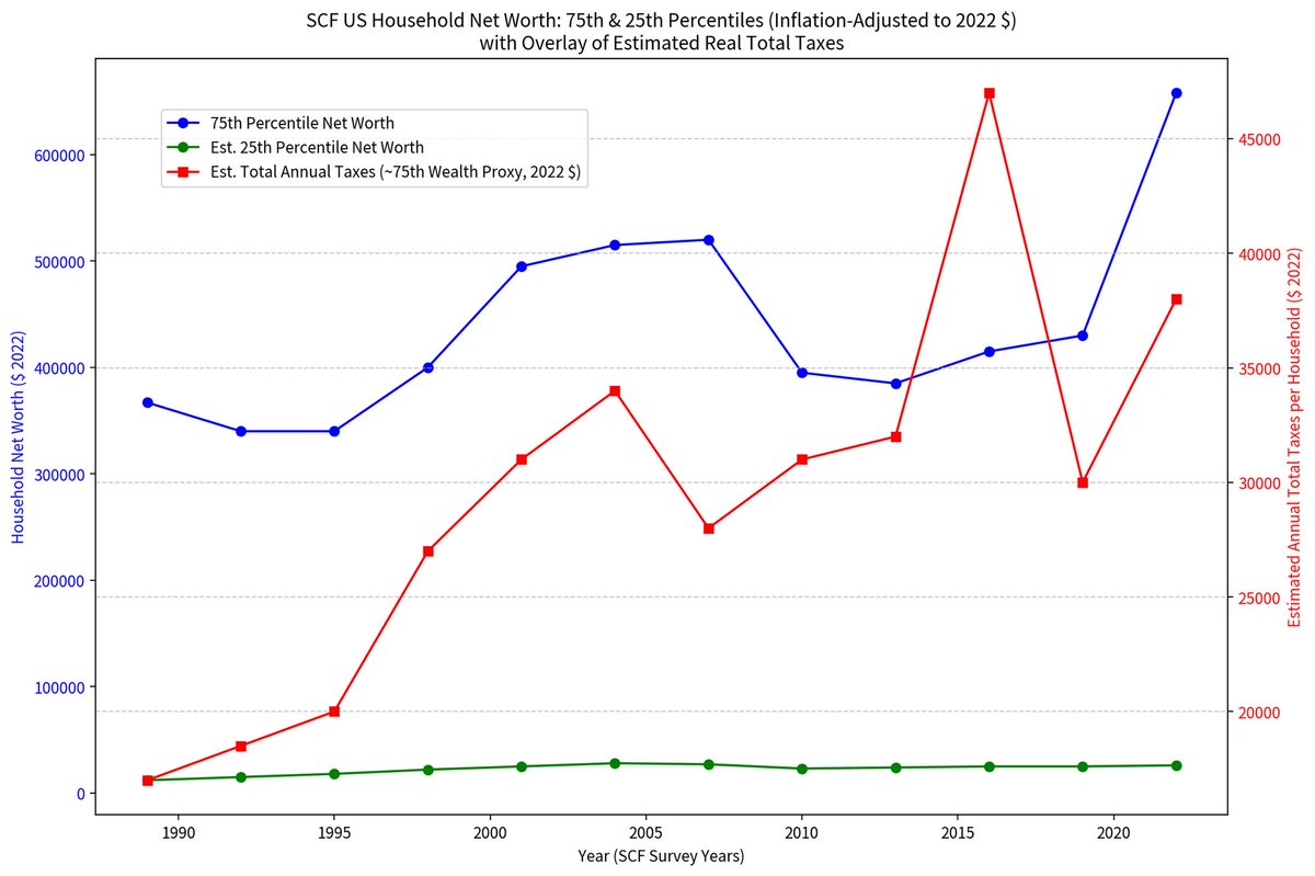
@BobClimko The Gini coefficient is more sensational and less informative. The SCF looks at the gaps between 25%tile and 75%tile as shown. The poor have always been about the same. The 75% have increased and this includes house wealth etc.
Intracra pressure (ICP) equations for steady-state and dynamic prediction of responses to neuro-critical disease processes, pharmacologic and surgical interventions. Repurposed from https://t.co/dfk8Jeg4AM
The retina does employ a mechanism that results in focal suppression of activity in certain ganglion cells around high-intensity (bright) areas, though it’s not a specialized “anti-glare” system but part of the standard center-surround organization and lateral inhibition.3257
This works through the receptive fields of retinal ganglion cells (RGCs), the output neurons of the retina that send visual signals to the brain via the optic nerve. Most RGCs have center-surround receptive fields with antagonistic (opposing) responses:
•On-center/off-surround RGCs: Excited by bright light in the center of their receptive field; inhibited by bright light in the surrounding ring.
•Off-center/on-surround RGCs: The opposite pattern.
This antagonism arises from lateral inhibition, mediated primarily by horizontal cells (in the outer retina) and amacrine cells (in the inner retina). When a high-intensity bright spot or “glared” area stimulates photoreceptors in one region, it strongly activates the centers of RGCs directly under it (boosting their firing if on-center). However, it simultaneously stimulates the surrounds of neighboring RGCs whose centers are just outside the bright area. This causes inhibition/suppression of those adjacent ganglion cells.4653
In effect:
•The retina emphasizes contrast and edges around the bright region (e.g., making boundaries sharper, as in Mach bands illusions).
•It relatively suppresses responses in the immediate surrounding retinal areas to uniform or diffuse bright light.
•This helps the visual system handle wide ranges of luminance without saturation and downplays uniform background illumination.37
Important caveats regarding “glare” specifically:
•True glare/halos around bright lights (e.g., headlights at night or high-intensity projected images) are mostly caused by optical scattering of light in the eye’s cornea, lens, or vitreous before it reaches the retina—not by retinal processing itself.
•The retina processes whatever light pattern actually arrives on the photoreceptors. Lateral inhibition enhances perceived contrast within that pattern but does not eliminate or actively “cancel” scattered light halos.
•Some specialized RGC types (e.g., certain direction-selective or suppressed-by-contrast cells) show additional luminance suppression under specific conditions, but the core center-surround mechanism applies broadly.56
This retinal strategy is highly efficient for edge detection and adaptation but is why we still perceive halos or reduced visibility around intense lights when scatter is high (e.g., cataracts, aging eyes). It is not identical to artificial systems like certain image-processing algorithms or display tech that might explicitly mask or suppress around glare sources, but it achieves a functionally similar local contrast enhancement via biological “focal suppression” of nearby ganglion cell activity.
In short, yes—the retina uses this built-in suppression around high-intensity regions as a core part of how it sharpens vision.
Photon count image reconstruction (as used in Tesla’s FSD context) primarily improves handling of high-dynamic-range (HDR) scenes with intense light sources, such as direct sun or headlights, by bypassing traditional image signal processing (ISP) that exacerbates glare and scatter effects. It does not physically eliminate Mie scattering but enables better recovery of scene details despite it.56
What is Mie Scattering in This Context?
Mie scattering occurs when light interacts with particles (e.g., water droplets in fog/haze, dust, or aerosols) roughly the size of the light’s wavelength or larger. It is strongly forward-directed (unlike Rayleigh scattering) and creates:
•Haze, veiling glare, or bloom in images.
•Scattered photons that mix with direct light from the scene, reducing contrast and washing out details, especially in bright conditions where intense sources amplify the effect.74
In cameras, this combines with optical effects (lens flare, sensor bloom) and ISP artifacts.
How Traditional Cameras/Processing Handle (and Worsen) It
Standard RGB cameras use:
•Fixed or auto exposure over an integration time → Bright sources saturate pixels (clip to maximum value), spreading charge or causing bloom.
•Image Signal Processor (ISP) steps: demosaicing, white balance, tone mapping, gamma correction, compression. These often average, clip, or compress dynamic range to fit 8-bit outputs, amplifying scattered light’s veiling effect and losing faint signals in darker areas.37
Result: A “washed-out” image where glare from Mie-scattered light (or direct bright sources) obscures roads, vehicles, etc.
How Photon Count Reconstruction Works and Reduces the Impact
Tesla’s approach (direct/raw photon counting) feeds high-fidelity raw sensor data to the neural net:
1Raw Photon Detection: Sensors (CMOS photodiodes) convert photons to charge linearly. Instead of long exposures + ISP, the system uses very short integration times or high-frame-rate captures to avoid saturation even in bright sunlight. Each “frame” records precise photon counts per pixel (or near-single-photon sensitivity in aggregate).65
2Bypassing ISP: Raw counts (high dynamic range, often effectively 16+ bits or more via temporal integration) go directly to the NN. No early clipping, tone mapping, or averaging that mixes scattered photons indiscriminately with scene signals.56
3Neural Reconstruction:
◦The NN learns to interpret photon statistics across space and time.
◦It can separate direct (ballistic) photons from scattered ones using patterns, motion, multi-frame fusion, and learned priors about the world (e.g., road geometry, object consistency).
◦Temporal fusion (short exposures summed intelligently) preserves faint details in low-light areas while handling bright ones without global washout.
◦This yields HDR-like reconstruction: clear houses, cars, trees, etc., even when standard RGB looks blown out.10
Key advantage against Mie scatter: Scattered light adds a low-frequency veil or noise. With raw counts and no lossy processing, the NN can model and subtract this veil more effectively (similar to computational dehazing or time-of-flight separation in research, though Tesla relies on vision + learning rather than explicit pulsed lasers). Short exposures also limit the accumulation of scattered photons per frame.8
In essence, it’s not active scatter removal (like anti-scatter grids in CT or coherence gating) but preservation of information so the AI can reconstruct the underlying scene. Traditional processing destroys that info early; photon-to-NN keeps it.81
This aligns with Tesla’s “photon-to-control” philosophy: minimal processing until the end-to-end neural model. Real-world gains are most visible in glare, night, or haze, where human-like (or better) perception emerges from the data. Limitations remain (e.g., extreme fog may still challenge pure vision), but it represents a major edge over standard camera pipelines.
Glaucoma Broken-stick analysis reveals a higher, more actionable IOP threshold with CATS (21 mmHg, ~10× faster RNFL thinning above threshold) compared to Goldmann tonometry (18.5 mmHg, ~3.5× acceleration). Data from same-visit measurements in ~150 eyes.
These non-intuitive orbits (L1-L5) are Eigen value solutions to a 5th order polynomial describing 3 body orbits. Shown are the point solutions where stable satellites could be placed. Also their rotation can be in the same plane as the earth-sun or 90 degrees to it.
Interesting non-intuitive satellite orbits (we always think of them circling a body). The Webb telescope orbits an ethereal point (L2) about 1.5M km beyond the earth's path and out of the plane of planetary rotation as shown.
My understanding is that the oblique shocks increase the pressure on the back-side of the cone actually pulling the engine forward and the variable cone position along with flow vents are used to maintain the shocks which produce about 60% of the thrust. Also a supersonic flow bypass is used to produce a ram jet configuration around the subsonic combustion chamber. Absolutely amazing.
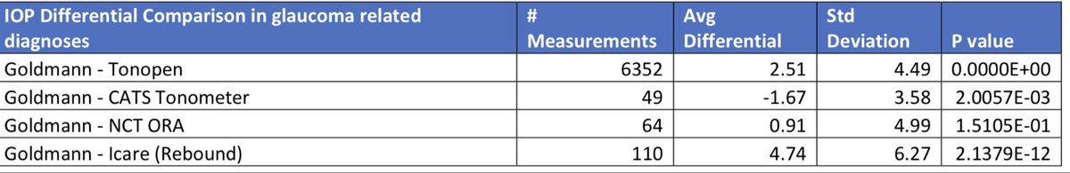
Last year we had 4000 glaucoma related IOP visits which produced 1/4 million lines of data on Mod Med. Grok wrote the software to distill the data down the following table in about 1.5hrs. Tonopen about +1 to -6mmHg lower than Goldmann, CATS higher on average, ORA about the same but more random and iCare was low and the most random.
The verbiage is somewhat convoluted. The table is correct. The beauty of AI is anyone can now do almost instantly do what literally took a coding consultant. The was done as a test. I plan to crunch 7+ years and probable 5 million lines of data. This tool increases my productivity by 10-100x.
Last year we had 4000 glaucoma related IOP visits which produced 1/4 million lines of data on Mod Med. Grok wrote the software to distill the data down the following table in about 1.5hrs. Tonopen about +1 to -6mmHg lower than Goldmann, CATS higher on average, ORA about the same but more random and iCare was low and the most random.