What is AdaBoost? (in ML interviews)
👋 Let's learn together ↓
𝗔𝗱𝗮𝗕𝗼𝗼𝘀𝘁 𝗶𝘀 𝗮𝗻 𝗲𝗻𝘀𝗲𝗺𝗯𝗹𝗲 𝗺𝗲𝘁𝗵𝗼𝗱 𝘁𝗵𝗮𝘁 𝗰𝗼𝗺𝗯𝗶𝗻𝗲𝘀 𝘄𝗲𝗮𝗸 𝗹𝗲𝗮𝗿𝗻𝗲𝗿𝘀 𝗶𝗻𝘁𝗼 𝗮 𝘀𝘁𝗿𝗼𝗻𝗴 𝗰𝗹𝗮𝘀𝘀𝗶𝗳𝗶𝗲𝗿.
It trains models sequentially. Each new model focuses on the mistakes of the previous ones by giving misclassified samples higher weight.
Think: a team where each member specializes in fixing what others got wrong.
📐 𝗧𝗵𝗲 𝗳𝗶𝗻𝗮𝗹 𝗺𝗼𝗱𝗲𝗹:
H(x) = sign(Σ αt ht(x)) for t=1 to T
Where:
T → number of weak learners
ht(x) → prediction from learner t
αt → learner weight (higher for better performers)
⚡ 𝗛𝗼𝘄 𝗶𝘁 𝘁𝗿𝗮𝗶𝗻𝘀:
① Start with equal sample weights
② Train weak learner on weighted data
③ Calculate learner weight: αt = ½ ln((1-εt)/εt) where εt is error rate
④ Update sample weights: increase weight on misclassified points by e^(αt·yi·ht(xi))
⑤ Normalize weights and repeat
Each round makes hard examples harder to ignore.
🧐 𝗛𝗼𝘄 𝗶𝘀 𝗶𝘁 𝗱𝗶𝗳𝗳𝗲𝗿𝗲𝗻𝘁 𝗳𝗿𝗼𝗺 𝗚𝗿𝗮𝗱𝗶𝗲𝗻𝘁 𝗕𝗼𝗼𝘀𝘁𝗶𝗻𝗴?
AdaBoost adjusts sample weights and uses exponential loss. Each learner sees a reweighted dataset.
Gradient Boosting fits residuals directly and works with any differentiable loss. Each learner corrects the previous ensemble's errors.
AdaBoost is simpler but less flexible. Gradient Boosting handles regression and custom losses better.
✍️ 𝗪𝗵𝗲𝗻 𝘁𝗼 𝘂𝘀𝗲 𝗔𝗱𝗮𝗕𝗼𝗼𝘀𝘁:
when you have weak learners (like shallow trees), need a simple boosting baseline, or want interpretable learner weights showing which models matter most.
👉 Land Data & AI jobs on https://t.co/B83Otkqc2r
What is Precision, Recall & F1 Score? (in ML interviews)
👋 Let's learn together ↓
𝗣𝗿𝗲𝗰𝗶𝘀𝗶𝗼𝗻, 𝗥𝗲𝗰𝗮𝗹𝗹, 𝗮𝗻𝗱 𝗙𝟭 𝗦𝗰𝗼𝗿𝗲 𝗮𝗿𝗲 𝗺𝗲𝘁𝗿𝗶𝗰𝘀 𝘁𝗵𝗮𝘁 𝗺𝗲𝗮𝘀𝘂𝗿𝗲 𝗰𝗹𝗮𝘀𝘀𝗶𝗳𝗶𝗲𝗿 𝗽𝗲𝗿𝗳𝗼𝗿𝗺𝗮𝗻𝗰𝗲 𝗯𝗲𝘆𝗼𝗻𝗱 𝗮𝗰𝗰𝘂𝗿𝗮𝗰𝘆.
Accuracy can be misleading when classes are imbalanced. If 95% of emails are not spam, a model that always predicts "not spam" gets 95% accuracy but catches zero spam.
Precision and Recall expose this. They measure different types of errors and force you to think about the trade-off between false positives and false negatives.
📐 𝗧𝗵𝗲 𝗳𝗼𝗿𝗺𝘂𝗹𝗮𝘀:
Precision = TP / (TP + FP)
Recall = TP / (TP + FN)
F1 Score = 2 × (Precision × Recall) / (Precision + Recall)
Where:
TP → True Positives (correctly predicted positive)
FP → False Positives (predicted positive, actually negative)
FN → False Negatives (predicted negative, actually positive)
TN → True Negatives (correctly predicted negative)
⚡ 𝗪𝗵𝗮𝘁 𝘁𝗵𝗲𝘆 𝗺𝗲𝗮𝘀𝘂𝗿𝗲:
𝗣𝗿𝗲𝗰𝗶𝘀𝗶𝗼𝗻: Of all predicted positives, how many are actually positive?
High precision means few false alarms. Use when false positives are expensive (spam filter blocking real emails).
𝗥𝗲𝗰𝗮𝗹𝗹: Of all actual positives, how many did we catch?
High recall means few missed cases. Use when false negatives are expensive (cancer screening missing a tumor).
𝗙𝟭 𝗦𝗰𝗼𝗿𝗲: Harmonic mean of precision and recall.
Balances both metrics. Good when you care about both types of errors equally.
🎯 𝗧𝗵𝗲 𝘁𝗿𝗮𝗱𝗲-𝗼𝗳𝗳:
You can't maximize both at once.
Lower your classification threshold and recall goes up (catch more positives) but precision drops (more false alarms).
Raise the threshold and precision improves but recall falls (miss real cases).
The precision-recall curve shows this relationship. Pick the threshold that matches your business cost.
🧐 𝗛𝗼𝘄 𝗶𝘀 𝗙𝟭 𝗱𝗶𝗳𝗳𝗲𝗿𝗲𝗻𝘁 𝗳𝗿𝗼𝗺 𝗔𝗰𝗰𝘂𝗿𝗮𝗰𝘆?
Accuracy treats all errors the same and breaks on imbalanced data.
F1 focuses only on the positive class and penalizes extreme imbalance between precision and recall.
F1 uses harmonic mean (not arithmetic), so if either precision or recall is low, F1 is low.
Accuracy can be high even when your model is useless for the minority class.
✍️ 𝗪𝗵𝗲𝗻 𝘁𝗼 𝘂𝘀𝗲 𝘁𝗵𝗲𝘀𝗲 𝗺𝗲𝘁𝗿𝗶𝗰𝘀:
when classes are imbalanced, when different errors have different costs, or when you need to justify your threshold choice in an interview.
👉 Land Data & AI jobs on https://t.co/B83Otkqc2r
What is a Confusion Matrix? (in ML interviews)
👋 Let's learn together ↓
A confusion matrix is a 𝘁𝗮𝗯𝗹𝗲 𝘁𝗵𝗮𝘁 𝘀𝗵𝗼𝘄𝘀 𝗵𝗼𝘄 𝘆𝗼𝘂𝗿 𝗰𝗹𝗮𝘀𝘀𝗶𝗳𝗶𝗲𝗿 𝗽𝗲𝗿𝗳𝗼𝗿𝗺𝗲𝗱 by comparing predictions to actual outcomes.
It's the foundation for understanding where your model succeeds and where it fails. Every classification metric (precision, recall, F1) comes from this table.
Think: a 2x2 grid that breaks down correct and incorrect predictions by class.
📐 𝗧𝗵𝗲 𝗺𝗮𝘁𝗿𝗶𝘅 𝘀𝘁𝗿𝘂𝗰𝘁𝘂𝗿𝗲:
Rows = Actual labels
Columns = Predicted labels
Four cells:
TP (True Positive) → predicted positive, actually positive
FP (False Positive) → predicted positive, actually negative
FN (False Negative) → predicted negative, actually positive
TN (True Negative) → predicted negative, actually negative
🧮 𝗞𝗲𝘆 𝗺𝗲𝘁𝗿𝗶𝗰𝘀 𝗱𝗲𝗿𝗶𝘃𝗲𝗱 𝗳𝗿𝗼𝗺 𝗶𝘁:
Precision = TP / (TP + FP)
→ of all positive predictions, how many were right?
Recall = TP / (TP + FN)
→ of all actual positives, how many did we catch?
F1 Score = 2 × (Precision × Recall) / (Precision + Recall)
→ harmonic mean balancing both
Accuracy = (TP + TN) / (TP + TN + FP + FN)
→ overall correctness (misleading on imbalanced data)
⚡ 𝗛𝗼𝘄 𝘁𝗼 𝗿𝗲𝗮𝗱 𝗶𝘁:
① Look at the diagonal (TP and TN). These are correct predictions.
② Check FP. These are false alarms (Type I error).
③ Check FN. These are missed cases (Type II error).
④ Calculate metrics based on what matters for your problem.
🔍 𝗛𝗼𝘄 𝗶𝘀 𝗶𝘁 𝗱𝗶𝗳𝗳𝗲𝗿𝗲𝗻𝘁 𝗳𝗿𝗼𝗺 𝗮𝗰𝗰𝘂𝗿𝗮𝗰𝘆 𝗮𝗹𝗼𝗻𝗲?
Accuracy gives you one number. Looks great on balanced data but hides problems on imbalanced sets.
A confusion matrix shows you exactly which errors you're making. You can see if you're missing positives (low recall) or getting too many false alarms (low precision).
It tells the full story. Accuracy just gives the summary.
✍️ 𝗪𝗵𝗲𝗻 𝘁𝗼 𝘂𝘀𝗲 𝗮 𝗖𝗼𝗻𝗳𝘂𝘀𝗶𝗼𝗻 𝗠𝗮𝘁𝗿𝗶𝘅:
every time you evaluate a classifier. It's the first thing you should check to understand model behavior and pick the right metric for your business problem.
👉 Land Data & AI jobs on https://t.co/B83Otkqc2r
What is Selection Bias? (in A/B test interviews)
👋 Let's learn together ↓
𝗦𝗲𝗹𝗲𝗰𝘁𝗶𝗼𝗻 𝗯𝗶𝗮𝘀 𝗼𝗰𝗰𝘂𝗿𝘀 𝘄𝗵𝗲𝗻 𝘆𝗼𝘂𝗿 𝘀𝗮𝗺𝗽𝗹𝗲 𝘀𝘆𝘀𝘁𝗲𝗺𝗮𝘁𝗶𝗰𝗮𝗹𝗹𝘆 𝗱𝗶𝗳𝗳𝗲𝗿𝘀 𝗳𝗿𝗼𝗺 𝘁𝗵𝗲 𝗽𝗼𝗽𝘂𝗹𝗮𝘁𝗶𝗼𝗻.
Your estimates become wrong even if your model is perfect. The data you observe doesn't represent the reality you care about.
Example: if only high-performing users complete your survey, their average satisfaction will be higher than the true population mean. That gap is selection bias.
📐 𝗧𝗵𝗲 𝗺𝗮𝘁𝗵:
Bias = E[θ̂ₛ] - θ = E[θ | S = 1] - E[θ]
Where:
θ̂ₛ → estimate from selected sample
θ → true population parameter
S = 1 → indicator that unit was selected
E[θ | S = 1] → expected value in selected sample
⚡ 𝗛𝗼𝘄 𝗶𝘁 𝗵𝗮𝗽𝗽𝗲𝗻𝘀:
① Sample selection depends on outcome or related variables
② Observed distribution shifts away from population
③ Estimates calculated on biased sample
④ Results don't generalize to target population
Common causes: non-random sampling, survivorship (only seeing successes), missing data that's not random, conditioning on a collider variable.
🔍 𝗛𝗼𝘄 𝗶𝘀 𝗶𝘁 𝗱𝗶𝗳𝗳𝗲𝗿𝗲𝗻𝘁 𝗳𝗿𝗼𝗺 𝗦𝗮𝗺𝗽𝗹𝗶𝗻𝗴 𝗘𝗿𝗿𝗼𝗿?
Sampling error is random variation from taking a sample. It decreases with larger samples and averages out to zero.
Selection bias is systematic. It doesn't disappear with more data. Your sample is fundamentally unrepresentative, so adding more biased observations just gives you more confident wrong answers.
🧮 𝗖𝗼𝗿𝗿𝗲𝗰𝘁𝗶𝗼𝗻 𝗺𝗲𝘁𝗵𝗼𝗱𝘀:
Heckman correction models the selection mechanism first, then adjusts outcome estimates.
Inverse probability weighting reweights observations by 1/P(selected) to recover population distribution.
Randomized designs with intent-to-treat analysis prevent selection by design.
✍️ 𝗪𝗵𝗲𝗻 𝘁𝗼 𝘄𝗮𝘁𝗰𝗵 𝗳𝗼𝗿 𝗦𝗲𝗹𝗲𝗰𝘁𝗶𝗼𝗻 𝗕𝗶𝗮𝘀:
whenever participation is voluntary, data is missing non-randomly, or you're analyzing survivors (customers who didn't churn, products still in market, experiments that finished).
👉 Land Data & AI jobs on https://t.co/B83Otkqc2r
What is DBSCAN? (in ML interviews)
👋 Let's learn together ↓
DBSCAN is a 𝗱𝗲𝗻𝘀𝗶𝘁𝘆-𝗯𝗮𝘀𝗲𝗱 𝗰𝗹𝘂𝘀𝘁𝗲𝗿𝗶𝗻𝗴 𝗮𝗹𝗴𝗼𝗿𝗶𝘁𝗵𝗺 that finds clusters by linking points in dense neighborhoods.
No need to specify k upfront. Outliers fall out automatically as noise. It handles rings, moons, spirals. Things K-Means simply can't do.
The core idea: if enough points live within radius ε of a point, that point seeds a cluster and grows it outward by chaining dense neighborhoods together.
📐 𝗧𝗵𝗲 𝗰𝗼𝗿𝗲 𝗿𝘂𝗹𝗲:
Nε(p) = { q ∈ D : d(p, q) ≤ ε }
Where:
Nε(p) → all points within distance ε of point p
ε → neighborhood radius (you set this)
minPts → minimum neighbors needed to be a core point
Every point gets one of three roles:
🟢 𝗖𝗼𝗿𝗲 → has at least minPts neighbors within ε. Seeds and grows a cluster.
🔵 𝗕𝗼𝗿𝗱𝗲𝗿 → inside a core's ε-ball but not dense enough itself. Joins the cluster, never expands it.
🔴 𝗡𝗼𝗶𝘀𝗲 → unreachable from any core. Labeled -1. Free outlier detection.
💪 𝗛𝗼𝘄 𝗶𝘁 𝘄𝗼𝗿𝗸𝘀:
① Pick an unvisited point
② Check if it has ≥ minPts neighbors within ε
③ If yes, start a new cluster and add all neighbors to a queue
④ Expand by checking each queued point the same way
⑤ Repeat until all points are visited. Noise points get label -1.
Density-reachability is asymmetric. A border point can be reached from a core, but can't reach back. Density-connectivity is symmetric. Two points are in the same cluster if some core point density-reaches both.
🧐 𝗛𝗼𝘄 𝗶𝘀 𝗶𝘁 𝗱𝗶𝗳𝗳𝗲𝗿𝗲𝗻𝘁 𝗳𝗿𝗼𝗺 𝗞-𝗠𝗲𝗮𝗻𝘀?
K-Means needs k upfront, makes hard spherical assignments, and has no concept of outliers.
DBSCAN discovers cluster count from density, handles any shape, and labels noise points automatically.
K-Means breaks on rings and spirals. DBSCAN doesn't.
The tradeoff: DBSCAN struggles when clusters have very different densities. A single ε can't fit all scales at once. That's where 𝗛𝗗𝗕𝗦𝗖𝗔𝗡 and 𝗢𝗣𝗧𝗜𝗖𝗦 come in. They remove the single-ε limit entirely.
🎯 𝗧𝘂𝗻𝗶𝗻𝗴 𝘁𝗶𝗽𝘀:
minPts ≈ 2 × number of dimensions (or ln n for large datasets)
Pick ε at the knee of the k-distance plot. Scale your features first or distance metrics become meaningless.
✍️ 𝗪𝗵𝗲𝗻 𝘁𝗼 𝘂𝘀𝗲 𝗗𝗕𝗦𝗖𝗔𝗡:
when clusters are non-convex, you don't know k, or outlier detection matters. Switch to HDBSCAN if density varies a lot across clusters.
👉 Land Data & AI jobs on https://t.co/B83Otkqc2r
What is Adam Optimizer? (in ML interviews)
👋 Let's learn together ↓
Adam is an 𝗮𝗱𝗮𝗽𝘁𝗶𝘃𝗲 𝗹𝗲𝗮𝗿𝗻𝗶𝗻𝗴 𝗿𝗮𝘁𝗲 𝗼𝗽𝘁𝗶𝗺𝗶𝘇𝗲𝗿 that combines momentum with per-parameter learning rates.
It tracks two moving averages: one for gradients (momentum) and one for squared gradients (adaptive rates). This lets it move fast in consistent directions while taking smaller steps in noisy dimensions.
Think of it as SGD with momentum plus RMSprop's adaptive scaling.
📐 𝗧𝗵𝗲 𝘂𝗽𝗱𝗮𝘁𝗲 𝗿𝘂𝗹𝗲:
θ(t+1) = θ(t) - η / √(v̂(t) + ε) × m̂(t)
Where:
m(t) → first moment (momentum)
v(t) → second moment (squared gradients)
m̂(t), v̂(t) → bias-corrected estimates
η → learning rate (often 0.001)
β₁ → momentum decay (typically 0.9)
β₂ → second moment decay (typically 0.999)
ε → small constant for stability (1e-8)
⚡ 𝗛𝗼𝘄 𝗶𝘁 𝘄𝗼𝗿𝗸𝘀:
① Compute gradient g(t)
② Update first moment: m(t) = β₁m(t-1) + (1-β₁)g(t)
③ Update second moment: v(t) = β₂v(t-1) + (1-β₂)g(t)²
④ Correct bias: m̂(t) = m(t)/(1-β₁ᵗ), v̂(t) = v(t)/(1-β₂ᵗ)
⑤ Update parameters using corrected moments
🧐 𝗛𝗼𝘄 𝗶𝘀 𝗶𝘁 𝗱𝗶𝗳𝗳𝗲𝗿𝗲𝗻𝘁 𝗳𝗿𝗼𝗺 𝗦𝗚𝗗 𝘄𝗶𝘁𝗵 𝗠𝗼𝗺𝗲𝗻𝘁𝘂𝗺?
SGD+Momentum uses a fixed learning rate for all parameters and only tracks gradient momentum.
Adam adjusts learning rates per parameter based on gradient history and tracks both first and second moments. It needs less manual tuning but uses more memory.
SGD often needs careful learning rate schedules. Adam works out of the box with default hyperparameters.
✍️ 𝗪𝗵𝗲𝗻 𝘁𝗼 𝘂𝘀𝗲 𝗔𝗱𝗮𝗺:
when you want fast prototyping with minimal tuning, training transformers or RNNs, or working with sparse gradients and non-stationary objectives.
👉 Land Data & AI jobs on https://t.co/B83Otkqc2r
What is A/B Testing? (in data science interviews)
👋 Let's learn together ↓
A/B testing is a 𝘀𝘁𝗮𝘁𝗶𝘀𝘁𝗶𝗰𝗮𝗹 𝗺𝗲𝘁𝗵𝗼𝗱 𝘁𝗼 𝗰𝗼𝗺𝗽𝗮𝗿𝗲 𝘁𝘄𝗼 𝘃𝗮𝗿𝗶𝗮𝗻𝘁𝘀 and determine which performs better on a target metric.
You split users randomly into control (A) and treatment (B) groups, expose them to different versions, then measure if the difference in outcomes is real or just noise.
It's how companies decide whether a new feature actually improves conversion, retention, or revenue.
📐 𝗧𝗵𝗲 𝘁𝗲𝘀𝘁 𝘀𝘁𝗮𝘁𝗶𝘀𝘁𝗶𝗰:
Z = (p̂ᵦ - p̂ₐ) / sqrt(p̄(1-p̄)(1/nₐ + 1/nᵦ))
Where:
p̂ₐ, p̂ᵦ → observed conversion rates in each group
p̄ → pooled proportion under null hypothesis
nₐ, nᵦ → sample sizes per group
💪 𝗛𝗼𝘄 𝗶𝘁 𝘄𝗼𝗿𝗸𝘀:
① Define your metric and minimum detectable effect
② Calculate required sample size based on α (Type I error) and power
③ Randomly assign users to control or treatment
④ Run the test until you hit sample size
⑤ Compute Z-score and compare to critical value
⑥ Reject null if |Z| exceeds threshold, otherwise fail to reject
🧐 𝗛𝗼𝘄 𝗶𝘀 𝗶𝘁 𝗱𝗶𝗳𝗳𝗲𝗿𝗲𝗻𝘁 𝗳𝗿𝗼𝗺 𝗕𝗮𝘆𝗲𝘀𝗶𝗮𝗻 𝗔/𝗕?
Classical A/B gives you a binary decision (reject or not) based on p-values and requires fixed sample sizes.
Bayesian A/B gives you a probability distribution over the treatment effect, lets you stop early when confident, and directly answers "what's the chance B is better?"
Classical is easier to explain to stakeholders. Bayesian is more flexible but needs prior specification.
✍️ 𝗪𝗵𝗲𝗻 𝘁𝗼 𝘂𝘀𝗲 𝗔/𝗕 𝘁𝗲𝘀𝘁𝗶𝗻𝗴:
when you need to validate product changes with statistical confidence before rolling them out to everyone.
👉 Land Data & AI jobs on https://t.co/B83Otkqc2r
What is Class Imbalance Handling? (in ML interviews)
👋 Let's learn together ↓
Class imbalance is when 𝗼𝗻𝗲 𝗰𝗹𝗮𝘀𝘀 𝗱𝗼𝗺𝗶𝗻𝗮𝘁𝗲𝘀 𝘁𝗵𝗲 𝗱𝗮𝘁𝗮 and the model learns to ignore the rare class entirely.
Say you have 190 majority points and 10 minority points. An unweighted model hits recall of 0.2 on the rare class. It's basically guessing majority every time. Reweight the loss, and recall jumps to 0.9. Same data, very different boundary.
The fix isn't one thing. It's a toolkit: reweight, resample, or shift the threshold.
📐 𝗧𝗵𝗲 𝗳𝗼𝗿𝗺𝘂𝗹𝗮𝘀:
𝗪𝗲𝗶𝗴𝗵𝘁𝗲𝗱 𝗟𝗼𝘀𝘀:
L = -(1/N) × sum of w_yi × [yi × log(p̂i) + (1 - yi) × log(1 - p̂i)]
Where:
w_yi → per-sample class weight, inflates rare-class gradients
yi → true label
p̂i → predicted probability
𝗜𝗻𝘃𝗲𝗿𝘀𝗲-𝗙𝗿𝗲𝗾𝘂𝗲𝗻𝗰𝘆 𝗪𝗲𝗶𝗴𝗵𝘁:
w_c = N / (K × N_c)
Where:
N → total samples
K → number of classes
N_c → samples in class c
𝗙𝗼𝗰𝗮𝗹 𝗟𝗼𝘀𝘀 (for dense/vision tasks):
FL(pt) = -αt × (1 - pt)^γ × log(pt)
Where:
(1 - pt)^γ → down-weights easy examples, focuses gradient on hard ones
αt → class balancing factor
γ → tunable focus parameter (RetinaNet uses γ=2)
💪 𝗛𝗼𝘄 𝘁𝗼 𝗮𝗽𝗽𝗹𝘆 𝗶𝘁 (𝗶𝗻 𝗼𝗿𝗱𝗲𝗿 𝗼𝗳 𝗲𝗳𝗳𝗼𝗿𝘁):
① Start with inverse-frequency weights. Pass class_weight to your loss. No resampling needed. Works well for tabular data with mild skew.
② Try SMOTE if weights aren't enough. It interpolates k-NN neighbors to synthesize minority samples. Only resample the training fold, never validation or test.
③ Tune the decision threshold. Train on raw data, then move the cutoff from 0.5 to maximize F1 or recall on validation. Cost-sensitive: minimize C_FN × FN + C_FP × FP.
④ Use focal loss for dense prediction tasks like object detection. It ignores easy majority examples automatically.
⑤ Pick the right metrics. Drop accuracy entirely. A 99% majority predictor scores 99% accuracy and is useless. Use PR-AUC, F1, or recall@k instead. Stratify your CV folds so each fold preserves the base rate.
🧐 𝗥𝗲𝘀𝗮𝗺𝗽𝗹𝗶𝗻𝗴 𝘃𝘀 𝗥𝗲𝘄𝗲𝗶𝗴𝗵𝘁𝗶𝗻𝗴:
Resampling (SMOTE) changes the data itself. It can overfit in high dimensions and adds preprocessing complexity. Best for low-dimensional structured data.
Reweighting changes the loss function. It's cheap, simple, and doesn't touch the data distribution. Works with any model that accepts sample weights.
Threshold tuning doesn't change training at all. It just shifts where you draw the line at inference time. Useful when you have a cost asymmetry between false positives and false negatives.
✍️ 𝗪𝗵𝗲𝗻 𝘁𝗼 𝘂𝘀𝗲 𝗖𝗹𝗮𝘀𝘀 𝗜𝗺𝗯𝗮𝗹𝗮𝗻𝗰𝗲 𝗛𝗮𝗻𝗱𝗹𝗶𝗻𝗴:
any time your rare class is the one that actually matters. Fraud detection, medical diagnosis, churn prediction. Start with reweighting, validate with PR-AUC, and tune the threshold last.
👉 Land Data & AI jobs on https://t.co/B83Otkqc2r
What is Ridge Regression? (in ML interviews)
👋 Let's learn together ↓
𝗥𝗶𝗱𝗴𝗲 𝗥𝗲𝗴𝗿𝗲𝘀𝘀𝗶𝗼𝗻 𝗶𝘀 𝗹𝗶𝗻𝗲𝗮𝗿 𝗿𝗲𝗴𝗿𝗲𝘀𝘀𝗶𝗼𝗻 𝘄𝗶𝘁𝗵 𝗟𝟮 𝗽𝗲𝗻𝗮𝗹𝘁𝘆.
It shrinks coefficients toward zero to fight overfitting and handle multicollinearity. Unlike Lasso, it never eliminates features completely. All coefficients stay in the model, just smaller.
Think: gentle pressure on all weights instead of aggressive feature selection.
📐 𝗧𝗵𝗲 𝗼𝗯𝗷𝗲𝗰𝘁𝗶𝘃𝗲:
β̂ridge = argmin { Σ(yi - Xiβ)² + λ Σβj² }
Where:
Σ(yi - Xiβ)² → RSS (residual sum of squares)
λ Σβj² → L2 penalty on coefficient magnitudes
λ → regularization strength (controls shrinkage)
💪 𝗛𝗼𝘄 𝗶𝘁 𝘄𝗼𝗿𝗸𝘀:
① Start with ordinary least squares setup
② Add penalty term that grows with coefficient size
③ Solve closed-form: β̂ = (XᵀX + λI)⁻¹Xᵀy
④ Tune λ via cross-validation to balance bias and variance
The λI term guarantees invertibility even when features are collinear. This stabilizes estimates.
🧐 𝗛𝗼𝘄 𝗶𝘀 𝗶𝘁 𝗱𝗶𝗳𝗳𝗲𝗿𝗲𝗻𝘁 𝗳𝗿𝗼𝗺 𝗟𝗮𝘀𝘀𝗼?
Lasso uses L1 penalty (absolute values) and drives some coefficients exactly to zero. It does feature selection.
Ridge uses L2 penalty (squared values) and shrinks all coefficients but keeps them nonzero. It keeps all features.
Lasso is sparse. Ridge is smooth.
✍️ 𝗪𝗵𝗲𝗻 𝘁𝗼 𝘂𝘀𝗲 𝗥𝗶𝗱𝗴𝗲:
when you have correlated features (r > 0.7), more features than samples, or unstable OLS estimates. Also when you want all features to contribute rather than selecting a subset.
👉 Land Data & AI jobs on https://t.co/B83Otkqc2r
What is Network Interference? (in A/B test interviews)
👋 Let's learn together ↓
Network interference happens when 𝘁𝗿𝗲𝗮𝘁𝗶𝗻𝗴 𝗼𝗻𝗲 𝘂𝘀𝗲𝗿 𝗮𝗳𝗳𝗲𝗰𝘁𝘀 𝗮𝗻𝗼𝘁𝗵𝗲𝗿 𝘂𝘀𝗲𝗿'𝘀 𝗼𝘂𝘁𝗰𝗼𝗺𝗲.
Standard A/B tests assume independence. But in social networks, marketplaces, or shared resources, users interact. Your treatment group influences your control group through connections.
This breaks SUTVA (Stable Unit Treatment Value Assumption) and makes naive estimates biased.
📐 𝗧𝗵𝗲 𝗽𝗿𝗼𝗯𝗹𝗲𝗺:
Yi(z) = Yi(zi, z-i) ≠ Yi(zi)
Where:
Yi(z) → outcome for unit i under assignment vector z
zi → treatment assigned to unit i
z-i → treatment assigned to all other units
The inequality shows unit i's outcome depends on others' assignments, violating independence.
⚡ 𝗧𝘆𝗽𝗲𝘀 𝗼𝗳 𝗶𝗻𝘁𝗲𝗿𝗳𝗲𝗿𝗲𝗻𝗰𝗲:
① Direct effect: treating unit i changes their own outcome
② Spillover effect: treating unit i changes connected units' outcomes
③ Contamination: control users get exposed through treated neighbors
Real example: you test a referral feature. Treated users invite control users. Control group gets the benefit without the treatment flag.
🎯 𝗛𝗼𝘄 𝘁𝗼 𝗺𝗲𝗮𝘀𝘂𝗿𝗲 𝗶𝘁:
Direct treatment effect = E[Yi(1,0) - Yi(0,0)]
Spillover effect = E[Yi(0,z_N) - Yi(0,0)]
First isolates individual impact. Second captures peer influence from having treated neighbors z_N.
🔍 𝗛𝗼𝘄 𝗶𝘀 𝗶𝘁 𝗱𝗶𝗳𝗳𝗲𝗿𝗲𝗻𝘁 𝗳𝗿𝗼𝗺 𝗿𝗲𝗴𝘂𝗹𝗮𝗿 𝗔/𝗕 𝘁𝗲𝘀𝘁𝘀?
Regular A/B tests assume treating one user doesn't affect others and randomize at the user level.
Network interference means users influence each other, requires cluster randomization (groups of connected users), and needs special estimators like Horvitz-Thompson to get unbiased effects.
Standard tests give you 30% upward bias from spillover contamination.
✍️ 𝗪𝗵𝗲𝗻 𝘁𝗼 𝘄𝗼𝗿𝗿𝘆 𝗮𝗯𝗼𝘂𝘁 𝗻𝗲𝘁𝘄𝗼𝗿𝗸 𝗶𝗻𝘁𝗲𝗿𝗳𝗲𝗿𝗲𝗻𝗰𝗲:
social features, marketplaces with supply/demand dynamics, shared inventory, pricing changes, or anything where users interact directly or compete for resources.
👉 Land Data & AI jobs on https://t.co/B83Otkqc2r
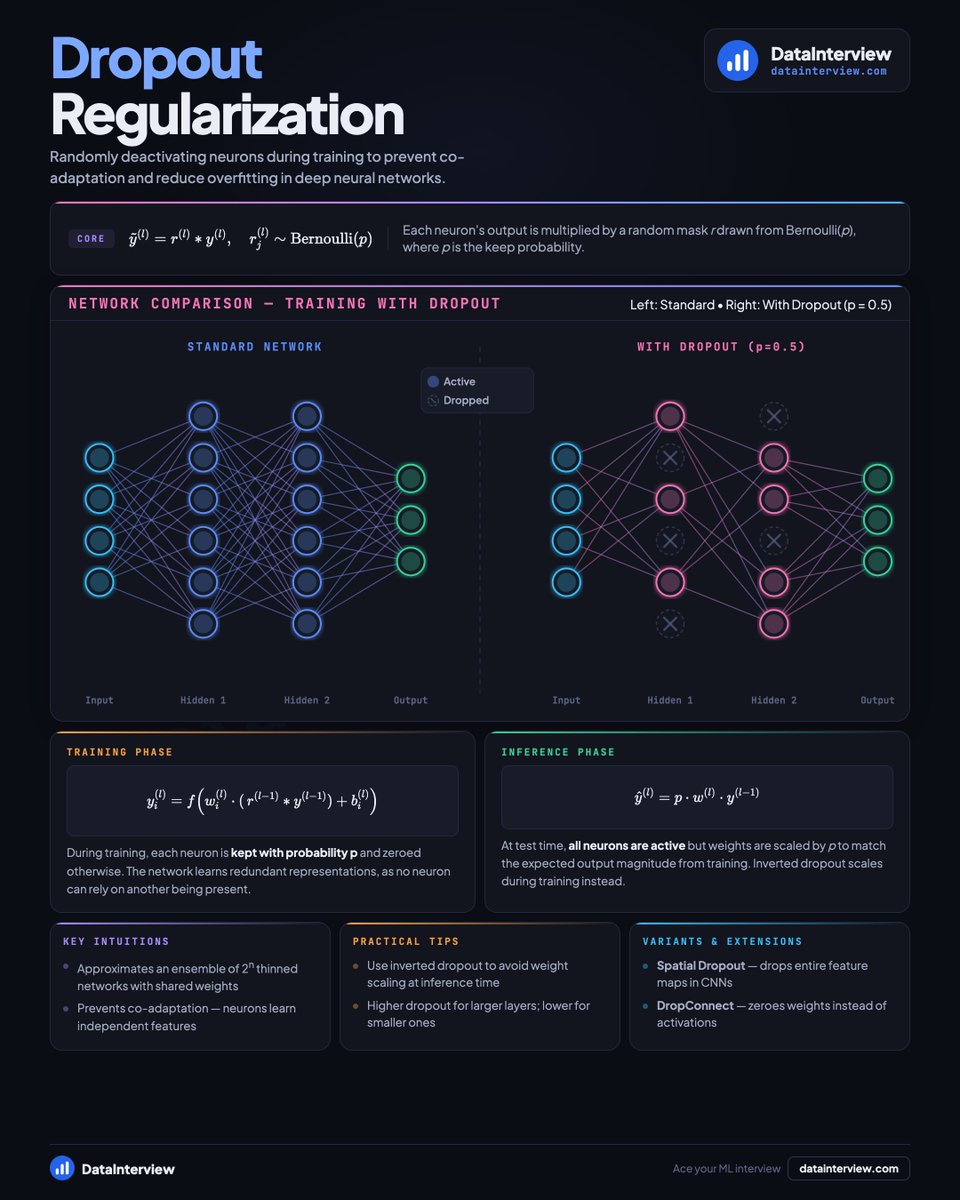
What is Dropout Regularization? (in ML interviews)
👋 Let's learn together ↓
Dropout is a 𝗿𝗲𝗴𝘂𝗹𝗮𝗿𝗶𝘇𝗮𝘁𝗶𝗼𝗻 𝘁𝗲𝗰𝗵𝗻𝗶𝗾𝘂𝗲 that randomly turns off neurons during training.
By forcing the network to learn without relying on any single neuron, it prevents co-adaptation (where neurons become too dependent on each other) and reduces overfitting.
Think of it like training a team where random members are absent each day. Everyone learns to be self-sufficient.
🧮 𝗧𝗵𝗲 𝗺𝗮𝘁𝗵:
ŷ⁽ˡ⁾ = r⁽ˡ⁾ * y⁽ˡ⁾
r⁽ˡ⁾ ~ Bernoulli(p)
Where:
y⁽ˡ⁾ → neuron activations at layer l
r⁽ˡ⁾ → binary mask (0 or 1 for each neuron)
p → keep probability (typically 0.5 for hidden layers)
* → element-wise multiplication
⚡ 𝗛𝗼𝘄 𝗶𝘁 𝘄𝗼𝗿𝗸𝘀:
① During training: randomly set each neuron to zero with probability (1-p)
② Active neurons pass their values forward normally
③ Backprop only updates weights connected to active neurons
④ At test time: use all neurons but scale outputs by p (or use inverted dropout to avoid this)
Each training batch sees a different "thinned" network.
🔍 𝗛𝗼𝘄 𝗶𝘀 𝗶𝘁 𝗱𝗶𝗳𝗳𝗲𝗿𝗲𝗻𝘁 𝗳𝗿𝗼𝗺 𝗟𝟮 𝗥𝗲𝗴𝘂𝗹𝗮𝗿𝗶𝘇𝗮𝘁𝗶𝗼𝗻?
L2 adds a penalty term to the loss function and shrinks all weights proportionally. It's deterministic.
Dropout randomly removes neurons during training and approximates training an ensemble of networks. It's stochastic and often works better for deep networks.
You can use both together.
✍️ 𝗪𝗵𝗲𝗻 𝘁𝗼 𝘂𝘀𝗲 𝗗𝗿𝗼𝗽𝗼𝘂𝘁:
when training deep networks prone to overfitting, especially with limited data. Higher rates (0.5) for large layers, lower (0.2) for smaller ones.
👉 Land Data & AI jobs on https://t.co/B83Otkqc2r
What is SHAP? (in ML interviews)
👋 Let's learn together ↓
SHAP is a 𝗴𝗮𝗺𝗲-𝘁𝗵𝗲𝗼𝗿𝗲𝘁𝗶𝗰 𝗳𝗿𝗮𝗺𝗲𝘄𝗼𝗿𝗸 𝗳𝗼𝗿 𝗲𝘅𝗽𝗹𝗮𝗶𝗻𝗶𝗻𝗴 𝗺𝗼𝗱𝗲𝗹 𝗽𝗿𝗲𝗱𝗶𝗰𝘁𝗶𝗼𝗻𝘀.
It answers: "how much did each feature contribute to this specific prediction?" It borrows from cooperative game theory, treating features as players sharing credit for the model's output.
The key insight: a feature's SHAP value is its average marginal contribution across every possible ordering of features. Fair, consistent, and model-agnostic.
📐 𝗧𝗵𝗲 𝗦𝗵𝗮𝗽𝗹𝗲𝘆 𝗳𝗼𝗿𝗺𝘂𝗹𝗮:
φᵢ = Σ [|S|!(|F|-|S|-1)! / |F|!] × [f(S∪{i}) - f(S)]
Where:
φᵢ → SHAP value for feature i
S → a coalition (subset) of other features
f(S∪{i}) - f(S) → marginal contribution of adding feature i to coalition S
|F| → total number of features
The sum of all SHAP values equals f(x) - E[f(X)]. That's the 𝗲𝗳𝗳𝗶𝗰𝗶𝗲𝗻𝗰𝘆 𝗮𝘅𝗶𝗼𝗺. Every bit of the prediction gap is explained.
🎯 𝗧𝗵𝗲 𝗳𝗼𝘂𝗿 𝗮𝘅𝗶𝗼𝗺𝘀:
① 𝗘𝗳𝗳𝗶𝗰𝗶𝗲𝗻𝗰𝘆: all SHAP values sum to f(x) - E[f(X)]
② 𝗦𝘆𝗺𝗺𝗲𝘁𝗿𝘆: two features with equal contributions get equal credit
③ 𝗗𝘂𝗺𝗺𝘆: a feature that changes nothing gets φ = 0
④ 𝗔𝗱𝗱𝗶𝘁𝗶𝘃𝗶𝘁𝘆: SHAP values from ensemble models can be summed across trees
These axioms make SHAP the only attribution method that satisfies all four simultaneously.
⚡ 𝗧𝗵𝗿𝗲𝗲 𝗺𝗮𝗶𝗻 𝗶𝗺𝗽𝗹𝗲𝗺𝗲𝗻𝘁𝗮𝘁𝗶𝗼𝗻𝘀:
① 𝗧𝗿𝗲𝗲𝗦𝗛𝗔𝗣: exact and fast for tree-based models (XGBoost, LightGBM). Use this by default for tabular data.
② 𝗗𝗲𝗲𝗽𝗦𝗛𝗔𝗣: approximation for neural networks using backprop. Fast but less exact.
③ 𝗞𝗲𝗿𝗻𝗲𝗹𝗦𝗛𝗔𝗣: model-agnostic. Fits a weighted linear surrogate around perturbed samples. Works on anything, but cost grows as 2^M so it's slow for many features.
🧐 𝗜𝗻𝘁𝗲𝗿𝘃𝗲𝗻𝘁𝗶𝗼𝗻𝗮𝗹 𝘃𝘀 𝗢𝗯𝘀𝗲𝗿𝘃𝗮𝘁𝗶𝗼𝗻𝗮𝗹 𝗦𝗛𝗔𝗣:
𝗜𝗻𝘁𝗲𝗿𝘃𝗲𝗻𝘁𝗶𝗼𝗻𝗮𝗹 marginalizes features independently. Causal-style. Can produce out-of-distribution inputs.
𝗢𝗯𝘀𝗲𝗿𝘃𝗮𝘁𝗶𝗼𝗻𝗮𝗹 respects feature correlations via the conditional distribution. Stays in-distribution, but splits credit strangely when features are correlated.
Correlated features are the hard part. Two correlated features can each get low SHAP values even if together they matter a lot. Prefer interventional SHAP when you want cleaner attribution and have correlated inputs.
✍️ 𝗪𝗵𝗲𝗻 𝘁𝗼 𝘂𝘀𝗲 𝗦𝗛𝗔𝗣:
when you need to explain individual predictions, debug a model, satisfy stakeholders, or compare global feature importance across a dataset by aggregating |φᵢ| values.
👉 Land Data & AI jobs on https://t.co/B83Otkqc2r
What is Metric Selection for A/B Tests? (in A/B test interviews)
👋 Let's learn together ↓
Metric selection is the 𝗽𝗿𝗼𝗰𝗲𝘀𝘀 𝗼𝗳 𝗰𝗵𝗼𝗼𝘀𝗶𝗻𝗴 𝗽𝗿𝗶𝗺𝗮𝗿𝘆, 𝗴𝘂𝗮𝗿𝗱𝗿𝗮𝗶𝗹, 𝗮𝗻𝗱 𝗱𝗶𝗮𝗴𝗻𝗼𝘀𝘁𝗶𝗰 𝗺𝗲𝘁𝗿𝗶𝗰𝘀 for an experiment.
You need to balance statistical sensitivity (can we detect a change?) with business alignment (does this metric actually matter?).
Pick wrong and you either run tests forever or ship changes that hurt the product.
📐 𝗧𝗵𝗲 𝘁𝗿𝗮𝗱𝗲𝗼𝗳𝗳:
Sensitivity vs. Business Alignment
High sensitivity → low variance, easy to detect changes, but might not reflect real value
High alignment → captures long-term impact, but noisy and needs huge samples
Sample size formula:
n = (Zα/2 + Zβ)² × 2σ² / δ²
Where:
Zα/2 → significance level (usually 1.96 for 95%)
Zβ → power (usually 0.84 for 80%)
σ² → metric variance
δ → minimum detectable effect
🎯 𝗧𝗵𝗲 𝗳𝗼𝘂𝗿 𝘁𝘆𝗽𝗲𝘀:
① 𝗣𝗿𝗶𝗺𝗮𝗿𝘆 (1 metric)
The single decision metric tied to your hypothesis.
Example: conversion rate for a checkout redesign.
② 𝗚𝘂𝗮𝗿𝗱𝗿𝗮𝗶𝗹 (2-4 metrics)
Must-not-harm constraints that protect the business.
Example: latency (p99) when testing a new recommendation model.
③ 𝗦𝗲𝗰𝗼𝗻𝗱𝗮𝗿𝘆 (3-5 metrics)
Explain the mechanism. No launch gate but help you understand why.
Example: CTR to explain why conversion changed.
④ 𝗗𝗶𝗮𝗴𝗻𝗼𝘀𝘁𝗶𝗰 (10+ metrics)
Debug and segment drill-down. Page views, error rates, cohort splits.
⚡ 𝗛𝗼𝘄 𝘁𝗼 𝗰𝗵𝗼𝗼𝘀𝗲:
① Start with business goal and map to metrics
② Calculate MDE for each candidate using variance and sample size
③ Pick primary with best sensitivity/alignment balance
④ Add guardrails for anything that could break
⑤ Pre-register everything to avoid p-hacking
🧐 𝗖𝗼𝗺𝗺𝗼𝗻 𝗺𝗶𝘀𝘁𝗮𝗸𝗲𝘀:
Using revenue-per-user as primary when you should use conversion rate (sensitivity matters).
Picking too many primaries without multiplicity correction (inflates false positives).
Choosing vanity metrics that move easily but don't correlate with long-term value.
Forgetting to check if your metric is actually movable by the treatment.
✍️ 𝗪𝗵𝗲𝗻 𝘁𝗼 𝘂𝘀𝗲 𝗠𝗲𝘁𝗿𝗶𝗰 𝗦𝗲𝗹𝗲𝗰𝘁𝗶𝗼𝗻:
before you run any A/B test. Pick metrics first, then design the experiment around them.
👉 Land Data & AI jobs on https://t.co/B83Otkqc2r
What is the Bias-Variance Tradeoff? (in ML interviews)
👋 Let's learn together ↓
The bias-variance tradeoff explains 𝘄𝗵𝘆 𝗺𝗼𝗱𝗲𝗹𝘀 𝗳𝗮𝗶𝗹 𝘁𝗼 𝗴𝗲𝗻𝗲𝗿𝗮𝗹𝗶𝘇𝗲 and how complexity affects prediction error.
Every model's error comes from three sources: bias (underfitting), variance (overfitting), and noise you can't avoid. You can't minimize both bias and variance at once. Reducing one increases the other.
This is the fundamental tension in machine learning.
📐 𝗧𝗵𝗲 𝗱𝗲𝗰𝗼𝗺𝗽𝗼𝘀𝗶𝘁𝗶𝗼𝗻:
Expected Error = Bias² + Variance + Irreducible Noise
Where:
Bias² → error from wrong assumptions (too simple)
Variance → error from sensitivity to training noise (too complex)
Irreducible Noise → randomness in data itself
⚡ 𝗛𝗼𝘄 𝗶𝘁 𝘄𝗼𝗿𝗸𝘀 (𝗮𝘀 𝗰𝗼𝗺𝗽𝗹𝗲𝘅𝗶𝘁𝘆 𝗶𝗻𝗰𝗿𝗲𝗮𝘀𝗲𝘀):
① Simple models: high bias, low variance (can't fit training data)
② Moderate models: bias and variance balanced (sweet spot)
③ Complex models: low bias, high variance (memorizes training noise)
④ Training error keeps dropping, but test error rises after the sweet spot
🧐 𝗛𝗼𝘄 𝗶𝘀 𝗼𝘃𝗲𝗿𝗳𝗶𝘁𝘁𝗶𝗻𝗴 𝗱𝗶𝗳𝗳𝗲𝗿𝗲𝗻𝘁 𝗳𝗿𝗼𝗺 𝘂𝗻𝗱𝗲𝗿𝗳𝗶𝘁𝘁𝗶𝗻𝗴?
Overfitting means training error is way lower than test error. The model memorized noise instead of patterns. High variance problem.
Underfitting means both errors stay high. The model is too simple to capture real patterns. High bias problem.
Fix overfitting by adding regularization, dropout, or more data. Fix underfitting by adding features, increasing model capacity, or training longer.
✍️ 𝗪𝗵𝗲𝗻 𝘁𝗼 𝘂𝘀𝗲 𝘁𝗵𝗶𝘀 𝗳𝗿𝗮𝗺𝗲𝘄𝗼𝗿𝗸:
when debugging why your model performs poorly, choosing model complexity, or explaining why cross-validation matters in interviews.
👉 Land Data & AI jobs on https://t.co/B83Otkqc2r
What is Gradient Boosting? (in ML interviews)
👋 Let's learn together ↓
Gradient Boosting is an 𝗲𝗻𝘀𝗲𝗺𝗯𝗹𝗲 𝗺𝗲𝘁𝗵𝗼𝗱 that builds a strong predictor by sequentially adding weak learners.
Each new model fits the negative gradient of the loss function. This means it corrects the errors of all previous models combined.
The result? A powerful additive model that improves step by step.
📐 𝗧𝗵𝗲 𝗰𝗼𝗿𝗲 𝘂𝗽𝗱𝗮𝘁𝗲:
Fm(x) = Fm-1(x) + ν · hm(x)
Where:
Fm(x) → ensemble prediction after m trees
hm(x) → new weak learner (usually a shallow tree)
ν → learning rate (controls step size)
Each tree fits pseudo-residuals, which are the negative gradient of the loss with respect to current predictions.
⚡ 𝗛𝗼𝘄 𝗶𝘁 𝘁𝗿𝗮𝗶𝗻𝘀:
① Start with an initial prediction (often the mean)
② Compute pseudo-residuals (negative gradient of loss)
③ Fit a weak learner to those residuals
④ Update the ensemble by adding the new tree (scaled by learning rate)
⑤ Repeat for M iterations
Loss decreases as the ensemble grows. Each tree corrects what came before.
🔍 𝗛𝗼𝘄 𝗶𝘀 𝗶𝘁 𝗱𝗶𝗳𝗳𝗲𝗿𝗲𝗻𝘁 𝗳𝗿𝗼𝗺 𝗥𝗮𝗻𝗱𝗼𝗺 𝗙𝗼𝗿𝗲𝘀𝘁?
Random Forest trains trees in parallel on bootstrapped samples and averages predictions. Trees are independent.
Gradient Boosting trains trees sequentially. Each tree depends on the errors of previous ones. It optimizes a loss function directly.
Random Forest reduces variance. Gradient Boosting reduces bias.
✍️ 𝗪𝗵𝗲𝗻 𝘁𝗼 𝘂𝘀𝗲 𝗚𝗿𝗮𝗱𝗶𝗲𝗻𝘁 𝗕𝗼𝗼𝘀𝘁𝗶𝗻𝗴:
when you need high accuracy on structured or tabular data and can afford careful tuning of depth and learning rate.
👉 Land Data & AI jobs on https://t.co/B83Otkqc2r
What is the Synthetic Control Method? (in A/B test interviews)
👋 Let's learn together ↓
Synthetic Control is a 𝗰𝗮𝘂𝘀𝗮𝗹 𝗶𝗻𝗳𝗲𝗿𝗲𝗻𝗰𝗲 𝗺𝗲𝘁𝗵𝗼𝗱 that builds a weighted combination of untreated units to mimic what would have happened to the treated unit without intervention.
You create a fake control group from real data. The weights are chosen so the synthetic control matches the treated unit's pre-treatment behavior as closely as possible.
Think: if you can't randomize, build the counterfactual yourself.
📐 𝗧𝗵𝗲 𝗺𝗼𝗱𝗲𝗹:
Ŷ₁ᴺ = Σ wⱼ Yⱼₜ for j=2 to J+1
Where:
Ŷ₁ᴺ → synthetic control outcome (what treated unit would've been)
wⱼ → donor weights (non-negative, sum to 1)
Yⱼₜ → observed outcomes from donor units
J → number of donor units
⚡ 𝗛𝗼𝘄 𝗶𝘁 𝘄𝗼𝗿𝗸𝘀:
① Collect pre-treatment data for treated unit and donor pool
② Solve optimization: minimize distance between treated unit's pre-treatment characteristics and weighted donors
③ Apply those same weights to post-treatment period
④ Treatment effect = actual outcome minus synthetic control outcome
🧐 𝗛𝗼𝘄 𝗶𝘀 𝗶𝘁 𝗱𝗶𝗳𝗳𝗲𝗿𝗲𝗻𝘁 𝗳𝗿𝗼𝗺 𝗗𝗶𝗳𝗳-𝗶𝗻-𝗗𝗶𝗳𝗳?
Diff-in-Diff uses parallel trends assumption and averages all control units equally.
Synthetic Control builds a custom weighted control, doesn't require parallel trends before treatment, and works with just one treated unit.
Diff-in-Diff needs multiple treated units for statistical power. Synthetic Control shines when you have one intervention (like a policy change in one state).
✍️ 𝗪𝗵𝗲𝗻 𝘁𝗼 𝘂𝘀𝗲 𝗦𝘆𝗻𝘁𝗵𝗲𝘁𝗶𝗰 𝗖𝗼𝗻𝘁𝗿𝗼𝗹:
when you have one treated unit, a long pre-treatment period, and a pool of similar untreated units to build your counterfactual from.
👉 Land Data & AI jobs on https://t.co/B83Otkqc2r
What is Bayesian Hyperparameter Tuning? (in ML interviews)
👋 Let's learn together ↓
Bayesian optimization is a 𝘀𝗺𝗮𝗿𝘁 𝘀𝗲𝗮𝗿𝗰𝗵 𝘀𝘁𝗿𝗮𝘁𝗲𝗴𝘆 that finds optimal hyperparameters using far fewer evaluations than grid or random search.
Instead of blindly testing combinations, it builds a probabilistic model of your objective function and intelligently picks the next point to try.
Think: learning from each experiment to guide the next one, not just guessing.
🧮 𝗧𝗵𝗲 𝗺𝗼𝗱𝗲𝗹 (𝗚𝗮𝘂𝘀𝘀𝗶𝗮𝗻 𝗣𝗿𝗼𝗰𝗲𝘀𝘀):
f(x) ~ GP(m(x), k(x, x'))
Where:
f(x) → your objective (validation accuracy, loss, etc.)
m(x) → mean prediction at point x
k(x, x') → covariance function (captures smoothness)
GP → gives both prediction and uncertainty at every point
⚡ 𝗛𝗼𝘄 𝗶𝘁 𝘄𝗼𝗿𝗸𝘀:
① Start with 5-10 random evaluations to initialize
② Fit a Gaussian Process to observed points
③ Use acquisition function to pick next point (balances exploration vs exploitation)
④ Evaluate objective at that point
⑤ Update GP with new observation
⑥ Repeat until budget exhausted or convergence
The acquisition function is key. Expected Improvement (EI) is most common:
EI(x) = E[max(0, f(x) - f(x*))]
Where:
f(x*) → current best observed value
EI → balances high mean (exploitation) with high variance (exploration)
🎯 𝗘𝘅𝗽𝗹𝗼𝗿𝗲 𝘃𝘀 𝗘𝘅𝗽𝗹𝗼𝗶𝘁:
The GP gives uncertainty estimates everywhere. High uncertainty means unexplored regions.
EI picks points that either look promising (high mean) or uncertain (high variance). This balance is automatic.
Grid search wastes time on bad regions. Bayesian opt learns to avoid them.
🔍 𝗛𝗼𝘄 𝗶𝘀 𝗶𝘁 𝗱𝗶𝗳𝗳𝗲𝗿𝗲𝗻𝘁 𝗳𝗿𝗼𝗺 𝗥𝗮𝗻𝗱𝗼𝗺 𝗦𝗲𝗮𝗿𝗰𝗵?
Random search samples uniformly without learning. Every trial is independent.
Bayesian optimization builds a model and uses past results to inform future choices. It concentrates trials in promising areas.
Random search needs hundreds of evaluations. Bayesian opt often finds good configs in 20-50 trials.
Random search works for any function. Bayesian opt assumes smoothness (nearby hyperparameters give similar performance).
✍️ 𝗪𝗵𝗲𝗻 𝘁𝗼 𝘂𝘀𝗲 𝗕𝗮𝘆𝗲𝘀𝗶𝗮𝗻 𝗛𝘆𝗽𝗲𝗿𝗽𝗮𝗿𝗮𝗺𝗲𝘁𝗲𝗿 𝗧𝘂𝗻𝗶𝗻𝗴:
when each evaluation is expensive (training deep nets, large datasets) and you need the best config with a limited budget. Tools like Optuna and HyperOpt make this easy.
👉 Land Data & AI jobs on https://t.co/B83Otkqc2r
What are Ensemble Methods? (in ML interviews)
👋 Let's learn together ↓
𝗘𝗻𝘀𝗲𝗺𝗯𝗹𝗲 𝗺𝗲𝘁𝗵𝗼𝗱𝘀 𝗰𝗼𝗺𝗯𝗶𝗻𝗲 𝗺𝘂𝗹𝘁𝗶𝗽𝗹𝗲 𝘄𝗲𝗮𝗸 𝗹𝗲𝗮𝗿𝗻𝗲𝗿𝘀 𝗶𝗻𝘁𝗼 𝗼𝗻𝗲 𝘀𝘁𝗿𝗼𝗻𝗴 𝗽𝗿𝗲𝗱𝗶𝗰𝘁𝗼𝗿.
Instead of trusting one model, you train many and aggregate their predictions. This reduces variance, bias, or both depending on the method.
Think: asking 100 people instead of 1 expert. The crowd's average is often better than any individual guess.
📐 𝗧𝗵𝗲 𝗳𝗼𝗿𝗺𝘂𝗹𝗮:
f̂(x) = Σ αm hm(x) for m=1 to M
Where:
M → number of base learners
hm(x) → prediction from model m
αm → weight for model m
f̂(x) → final ensemble prediction
⚡ 𝗧𝘄𝗼 𝗺𝗮𝗶𝗻 𝗮𝗽𝗽𝗿𝗼𝗮𝗰𝗵𝗲𝘀:
𝗕𝗮𝗴𝗴𝗶𝗻𝗴 (parallel training):
① Train M models on bootstrap samples (random subsets with replacement)
② Average predictions (regression) or vote (classification)
③ Reduces variance while keeping bias constant
④ Example: Random Forest
𝗕𝗼𝗼𝘀𝘁𝗶𝗻𝗴 (sequential training):
① Train model on full data
② Identify misclassified examples
③ Train next model focusing on those errors
④ Weight models by performance
⑤ Combine with weighted sum
⑥ Reduces bias primarily
⑦ Example: XGBoost, AdaBoost
🧐 𝗛𝗼𝘄 𝗶𝘀 𝗕𝗮𝗴𝗴𝗶𝗻𝗴 𝗱𝗶𝗳𝗳𝗲𝗿𝗲𝗻𝘁 𝗳𝗿𝗼𝗺 𝗕𝗼𝗼𝘀𝘁𝗶𝗻𝗴?
Bagging trains models independently in parallel on random subsets. It reduces variance. Works best with high-variance models like deep trees.
Boosting trains models sequentially where each corrects the previous one's mistakes. It reduces bias. Works best when you need to squeeze out every bit of accuracy.
✍️ 𝗪𝗵𝗲𝗻 𝘁𝗼 𝘂𝘀𝗲 𝗘𝗻𝘀𝗲𝗺𝗯𝗹𝗲𝘀:
when a single model isn't accurate enough, you have diverse base learners, or you're competing on Kaggle and need that extra 2% performance boost.
👉 Land Data & AI jobs on https://t.co/B83Otkqc2r
What is a Loss Function? (in ML interviews)
👋 Let's learn together ↓
A loss function is a 𝗺𝗮𝘁𝗵𝗲𝗺𝗮𝘁𝗶𝗰𝗮𝗹 𝗺𝗲𝗮𝘀𝘂𝗿𝗲 𝗼𝗳 𝗵𝗼𝘄 𝘄𝗿𝗼𝗻𝗴 𝘆𝗼𝘂𝗿 𝗺𝗼𝗱𝗲𝗹'𝘀 𝗽𝗿𝗲𝗱𝗶𝗰𝘁𝗶𝗼𝗻𝘀 𝗮𝗿𝗲.
It takes the difference between predicted and actual values, then converts that into a single number. The model's job during training? Make that number as small as possible.
Every gradient descent step moves in the direction that reduces this loss.
📐 𝗧𝗵𝗲 𝗴𝗲𝗻𝗲𝗿𝗮𝗹 𝗳𝗼𝗿𝗺:
ℒ(θ) = (1/N) × Σ L(yi, ŷi(θ)) for i=1 to N
Where:
yi → true label
ŷi → predicted value
θ → model parameters
L → per-sample loss function
⚡ 𝗛𝗼𝘄 𝗶𝘁 𝘄𝗼𝗿𝗸𝘀 (𝘁𝗿𝗮𝗶𝗻𝗶𝗻𝗴 𝗹𝗼𝗼𝗽):
① Forward pass: compute predictions ŷ
② Calculate loss: measure error between ŷ and y
③ Backward pass: compute gradients ∂ℒ/∂θ
④ Update parameters: θ = θ - α × gradient
⑤ Repeat until loss stops decreasing
🎯 𝗖𝗼𝗺𝗺𝗼𝗻 𝗹𝗼𝘀𝘀 𝗳𝘂𝗻𝗰𝘁𝗶𝗼𝗻𝘀:
MSE (Mean Squared Error):
ℒ = (1/N) × Σ(yi - ŷi)²
→ Penalizes large errors quadratically
→ Use for regression problems
→ Sensitive to outliers
Cross-Entropy:
ℒ = -(1/N) × Σ[yi ln ŷi + (1-yi) ln(1-ŷi)]
→ Measures probability divergence
→ Use for classification
→ Pairs with softmax outputs
MAE (Mean Absolute Error):
ℒ = (1/N) × Σ|yi - ŷi|
→ Linear penalty, more resistant to outliers
→ Gradient doesn't grow with error size
Huber Loss:
Combines MSE for small errors, MAE for large ones
→ Smooth everywhere with bounded gradients
→ Good middle ground for noisy data
🧐 𝗛𝗼𝘄 𝗶𝘀 𝗶𝘁 𝗱𝗶𝗳𝗳𝗲𝗿𝗲𝗻𝘁 𝗳𝗿𝗼𝗺 𝗮 𝗺𝗲𝘁𝗿𝗶𝗰?
Loss functions are differentiable and used during training to update weights. They need smooth gradients.
Metrics (like accuracy or F1) evaluate final performance but often aren't differentiable. You optimize the loss, then report the metric.
✍️ 𝗪𝗵𝗲𝗻 𝘁𝗼 𝗰𝗵𝗼𝗼𝘀𝗲 𝘄𝗵𝗶𝗰𝗵 𝗹𝗼𝘀𝘀:
match the loss to your problem type (regression vs classification), your data distribution (outliers?), and what errors matter most in your application.
👉 Land Data & AI jobs on https://t.co/B83Otkqc2r
What is a Switchback Experiment? (in A/B test interviews)
👋 Let's learn together ↓
A switchback experiment is a 𝘁𝗶𝗺𝗲-𝗯𝗮𝘀𝗲𝗱 𝗿𝗮𝗻𝗱𝗼𝗺𝗶𝘇𝗮𝘁𝗶𝗼𝗻 𝗱𝗲𝘀𝗶𝗴𝗻 for marketplace experiments.
Instead of assigning users to treatment or control, you alternate entire regions or markets between conditions over time. This solves interference problems when treating one user affects others.
Think: turning a feature on and off across different cities at different hours, not splitting individual riders.
📐 𝗧𝗵𝗲 𝗲𝘀𝘁𝗶𝗺𝗮𝘁𝗼𝗿:
τ̂ = (1/|T|) × Σ(Ȳt⁽¹⁾ - Ȳt⁽⁰⁾)
Where:
τ̂ → treatment effect estimate
|T| → number of time slots
Ȳt⁽¹⁾ → average outcome in treatment periods
Ȳt⁽⁰⁾ → average outcome in control periods
You difference within each region-time cell, then average.
⚡ 𝗛𝗼𝘄 𝗶𝘁 𝘄𝗼𝗿𝗸𝘀:
① Divide geography into regions (cities, zones, markets)
② Split time into slots (hours, days, weeks)
③ Randomly assign treatment/control to each region-time cell
④ Alternate assignments so each region sees both conditions
⑤ Measure outcomes and difference across matched time periods
The grid pattern balances time-of-day and day-of-week effects by design.
🧐 𝗛𝗼𝘄 𝗶𝘀 𝗶𝘁 𝗱𝗶𝗳𝗳𝗲𝗿𝗲𝗻𝘁 𝗳𝗿𝗼𝗺 𝘂𝘀𝗲𝗿-𝗹𝗲𝘃𝗲𝗹 𝗔/𝗕 𝘁𝗲𝘀𝘁𝘀?
User-level A/B tests randomize individuals and assume no spillover between users.
Switchback randomizes time-region blocks and handles network effects. It reduces bias when one user's treatment affects others (like surge pricing or driver supply). But it increases variance because you have fewer independent units.
Optimal slot length is usually 15-60 minutes. Too short and carryover effects bleed across periods. Too long and you lose statistical power.
✍️ 𝗪𝗵𝗲𝗻 𝘁𝗼 𝘂𝘀𝗲 𝘀𝘄𝗶𝘁𝗰𝗵𝗯𝗮𝗰𝗸𝘀:
when testing marketplace features like pricing, dispatch algorithms, or supply incentives where user-level randomization creates interference and biased estimates.
👉 Land Data & AI jobs on https://t.co/B83Otkqc2r


![datainterview's tweet photo. What is Selection Bias? (in A/B test interviews)
👋 Let's learn together ↓
𝗦𝗲𝗹𝗲𝗰𝘁𝗶𝗼𝗻 𝗯𝗶𝗮𝘀 𝗼𝗰𝗰𝘂𝗿𝘀 𝘄𝗵𝗲𝗻 𝘆𝗼𝘂𝗿 𝘀𝗮𝗺𝗽𝗹𝗲 𝘀𝘆𝘀𝘁𝗲𝗺𝗮𝘁𝗶𝗰𝗮𝗹𝗹𝘆 𝗱𝗶𝗳𝗳𝗲𝗿𝘀 𝗳𝗿𝗼𝗺 𝘁𝗵𝗲 𝗽𝗼𝗽𝘂𝗹𝗮𝘁𝗶𝗼𝗻.
Your estimates become wrong even if your model is perfect. The data you observe doesn't represent the reality you care about.
Example: if only high-performing users complete your survey, their average satisfaction will be higher than the true population mean. That gap is selection bias.
📐 𝗧𝗵𝗲 𝗺𝗮𝘁𝗵:
Bias = E[θ̂ₛ] - θ = E[θ | S = 1] - E[θ]
Where:
θ̂ₛ → estimate from selected sample
θ → true population parameter
S = 1 → indicator that unit was selected
E[θ | S = 1] → expected value in selected sample
⚡ 𝗛𝗼𝘄 𝗶𝘁 𝗵𝗮𝗽𝗽𝗲𝗻𝘀:
① Sample selection depends on outcome or related variables
② Observed distribution shifts away from population
③ Estimates calculated on biased sample
④ Results don't generalize to target population
Common causes: non-random sampling, survivorship (only seeing successes), missing data that's not random, conditioning on a collider variable.
🔍 𝗛𝗼𝘄 𝗶𝘀 𝗶𝘁 𝗱𝗶𝗳𝗳𝗲𝗿𝗲𝗻𝘁 𝗳𝗿𝗼𝗺 𝗦𝗮𝗺𝗽𝗹𝗶𝗻𝗴 𝗘𝗿𝗿𝗼𝗿?
Sampling error is random variation from taking a sample. It decreases with larger samples and averages out to zero.
Selection bias is systematic. It doesn't disappear with more data. Your sample is fundamentally unrepresentative, so adding more biased observations just gives you more confident wrong answers.
🧮 𝗖𝗼𝗿𝗿𝗲𝗰𝘁𝗶𝗼𝗻 𝗺𝗲𝘁𝗵𝗼𝗱𝘀:
Heckman correction models the selection mechanism first, then adjusts outcome estimates.
Inverse probability weighting reweights observations by 1/P(selected) to recover population distribution.
Randomized designs with intent-to-treat analysis prevent selection by design.
✍️ 𝗪𝗵𝗲𝗻 𝘁𝗼 𝘄𝗮𝘁𝗰𝗵 𝗳𝗼𝗿 𝗦𝗲𝗹𝗲𝗰𝘁𝗶𝗼𝗻 𝗕𝗶𝗮𝘀:
whenever participation is voluntary, data is missing non-randomly, or you're analyzing survivors (customers who didn't churn, products still in market, experiments that finished).
👉 Land Data & AI jobs on https://t.co/B83Otkqc2r](https://pbs.twimg.com/media/HInROS8XMAEiVPt.jpg)


![datainterview's tweet photo. What is Class Imbalance Handling? (in ML interviews)
👋 Let's learn together ↓
Class imbalance is when 𝗼𝗻𝗲 𝗰𝗹𝗮𝘀𝘀 𝗱𝗼𝗺𝗶𝗻𝗮𝘁𝗲𝘀 𝘁𝗵𝗲 𝗱𝗮𝘁𝗮 and the model learns to ignore the rare class entirely.
Say you have 190 majority points and 10 minority points. An unweighted model hits recall of 0.2 on the rare class. It's basically guessing majority every time. Reweight the loss, and recall jumps to 0.9. Same data, very different boundary.
The fix isn't one thing. It's a toolkit: reweight, resample, or shift the threshold.
📐 𝗧𝗵𝗲 𝗳𝗼𝗿𝗺𝘂𝗹𝗮𝘀:
𝗪𝗲𝗶𝗴𝗵𝘁𝗲𝗱 𝗟𝗼𝘀𝘀:
L = -(1/N) × sum of w_yi × [yi × log(p̂i) + (1 - yi) × log(1 - p̂i)]
Where:
w_yi → per-sample class weight, inflates rare-class gradients
yi → true label
p̂i → predicted probability
𝗜𝗻𝘃𝗲𝗿𝘀𝗲-𝗙𝗿𝗲𝗾𝘂𝗲𝗻𝗰𝘆 𝗪𝗲𝗶𝗴𝗵𝘁:
w_c = N / (K × N_c)
Where:
N → total samples
K → number of classes
N_c → samples in class c
𝗙𝗼𝗰𝗮𝗹 𝗟𝗼𝘀𝘀 (for dense/vision tasks):
FL(pt) = -αt × (1 - pt)^γ × log(pt)
Where:
(1 - pt)^γ → down-weights easy examples, focuses gradient on hard ones
αt → class balancing factor
γ → tunable focus parameter (RetinaNet uses γ=2)
💪 𝗛𝗼𝘄 𝘁𝗼 𝗮𝗽𝗽𝗹𝘆 𝗶𝘁 (𝗶𝗻 𝗼𝗿𝗱𝗲𝗿 𝗼𝗳 𝗲𝗳𝗳𝗼𝗿𝘁):
① Start with inverse-frequency weights. Pass class_weight to your loss. No resampling needed. Works well for tabular data with mild skew.
② Try SMOTE if weights aren't enough. It interpolates k-NN neighbors to synthesize minority samples. Only resample the training fold, never validation or test.
③ Tune the decision threshold. Train on raw data, then move the cutoff from 0.5 to maximize F1 or recall on validation. Cost-sensitive: minimize C_FN × FN + C_FP × FP.
④ Use focal loss for dense prediction tasks like object detection. It ignores easy majority examples automatically.
⑤ Pick the right metrics. Drop accuracy entirely. A 99% majority predictor scores 99% accuracy and is useless. Use PR-AUC, F1, or recall@k instead. Stratify your CV folds so each fold preserves the base rate.
🧐 𝗥𝗲𝘀𝗮𝗺𝗽𝗹𝗶𝗻𝗴 𝘃𝘀 𝗥𝗲𝘄𝗲𝗶𝗴𝗵𝘁𝗶𝗻𝗴:
Resampling (SMOTE) changes the data itself. It can overfit in high dimensions and adds preprocessing complexity. Best for low-dimensional structured data.
Reweighting changes the loss function. It's cheap, simple, and doesn't touch the data distribution. Works with any model that accepts sample weights.
Threshold tuning doesn't change training at all. It just shifts where you draw the line at inference time. Useful when you have a cost asymmetry between false positives and false negatives.
✍️ 𝗪𝗵𝗲𝗻 𝘁𝗼 𝘂𝘀𝗲 𝗖𝗹𝗮𝘀𝘀 𝗜𝗺𝗯𝗮𝗹𝗮𝗻𝗰𝗲 𝗛𝗮𝗻𝗱𝗹𝗶𝗻𝗴:
any time your rare class is the one that actually matters. Fraud detection, medical diagnosis, churn prediction. Start with reweighting, validate with PR-AUC, and tune the threshold last.
👉 Land Data & AI jobs on https://t.co/B83Otkqc2r](https://pbs.twimg.com/media/HISq6bSXAAEJmlB.jpg)

![datainterview's tweet photo. What is Network Interference? (in A/B test interviews)
👋 Let's learn together ↓
Network interference happens when 𝘁𝗿𝗲𝗮𝘁𝗶𝗻𝗴 𝗼𝗻𝗲 𝘂𝘀𝗲𝗿 𝗮𝗳𝗳𝗲𝗰𝘁𝘀 𝗮𝗻𝗼𝘁𝗵𝗲𝗿 𝘂𝘀𝗲𝗿'𝘀 𝗼𝘂𝘁𝗰𝗼𝗺𝗲.
Standard A/B tests assume independence. But in social networks, marketplaces, or shared resources, users interact. Your treatment group influences your control group through connections.
This breaks SUTVA (Stable Unit Treatment Value Assumption) and makes naive estimates biased.
📐 𝗧𝗵𝗲 𝗽𝗿𝗼𝗯𝗹𝗲𝗺:
Yi(z) = Yi(zi, z-i) ≠ Yi(zi)
Where:
Yi(z) → outcome for unit i under assignment vector z
zi → treatment assigned to unit i
z-i → treatment assigned to all other units
The inequality shows unit i's outcome depends on others' assignments, violating independence.
⚡ 𝗧𝘆𝗽𝗲𝘀 𝗼𝗳 𝗶𝗻𝘁𝗲𝗿𝗳𝗲𝗿𝗲𝗻𝗰𝗲:
① Direct effect: treating unit i changes their own outcome
② Spillover effect: treating unit i changes connected units' outcomes
③ Contamination: control users get exposed through treated neighbors
Real example: you test a referral feature. Treated users invite control users. Control group gets the benefit without the treatment flag.
🎯 𝗛𝗼𝘄 𝘁𝗼 𝗺𝗲𝗮𝘀𝘂𝗿𝗲 𝗶𝘁:
Direct treatment effect = E[Yi(1,0) - Yi(0,0)]
Spillover effect = E[Yi(0,z_N) - Yi(0,0)]
First isolates individual impact. Second captures peer influence from having treated neighbors z_N.
🔍 𝗛𝗼𝘄 𝗶𝘀 𝗶𝘁 𝗱𝗶𝗳𝗳𝗲𝗿𝗲𝗻𝘁 𝗳𝗿𝗼𝗺 𝗿𝗲𝗴𝘂𝗹𝗮𝗿 𝗔/𝗕 𝘁𝗲𝘀𝘁𝘀?
Regular A/B tests assume treating one user doesn't affect others and randomize at the user level.
Network interference means users influence each other, requires cluster randomization (groups of connected users), and needs special estimators like Horvitz-Thompson to get unbiased effects.
Standard tests give you 30% upward bias from spillover contamination.
✍️ 𝗪𝗵𝗲𝗻 𝘁𝗼 𝘄𝗼𝗿𝗿𝘆 𝗮𝗯𝗼𝘂𝘁 𝗻𝗲𝘁𝘄𝗼𝗿𝗸 𝗶𝗻𝘁𝗲𝗿𝗳𝗲𝗿𝗲𝗻𝗰𝗲:
social features, marketplaces with supply/demand dynamics, shared inventory, pricing changes, or anything where users interact directly or compete for resources.
👉 Land Data & AI jobs on https://t.co/B83Otkqc2r](https://pbs.twimg.com/media/HIIYcCHWYAAGEYB.jpg)
![datainterview's tweet photo. What is SHAP? (in ML interviews)
👋 Let's learn together ↓
SHAP is a 𝗴𝗮𝗺𝗲-𝘁𝗵𝗲𝗼𝗿𝗲𝘁𝗶𝗰 𝗳𝗿𝗮𝗺𝗲𝘄𝗼𝗿𝗸 𝗳𝗼𝗿 𝗲𝘅𝗽𝗹𝗮𝗶𝗻𝗶𝗻𝗴 𝗺𝗼𝗱𝗲𝗹 𝗽𝗿𝗲𝗱𝗶𝗰𝘁𝗶𝗼𝗻𝘀.
It answers: "how much did each feature contribute to this specific prediction?" It borrows from cooperative game theory, treating features as players sharing credit for the model's output.
The key insight: a feature's SHAP value is its average marginal contribution across every possible ordering of features. Fair, consistent, and model-agnostic.
📐 𝗧𝗵𝗲 𝗦𝗵𝗮𝗽𝗹𝗲𝘆 𝗳𝗼𝗿𝗺𝘂𝗹𝗮:
φᵢ = Σ [|S|!(|F|-|S|-1)! / |F|!] × [f(S∪{i}) - f(S)]
Where:
φᵢ → SHAP value for feature i
S → a coalition (subset) of other features
f(S∪{i}) - f(S) → marginal contribution of adding feature i to coalition S
|F| → total number of features
The sum of all SHAP values equals f(x) - E[f(X)]. That's the 𝗲𝗳𝗳𝗶𝗰𝗶𝗲𝗻𝗰𝘆 𝗮𝘅𝗶𝗼𝗺. Every bit of the prediction gap is explained.
🎯 𝗧𝗵𝗲 𝗳𝗼𝘂𝗿 𝗮𝘅𝗶𝗼𝗺𝘀:
① 𝗘𝗳𝗳𝗶𝗰𝗶𝗲𝗻𝗰𝘆: all SHAP values sum to f(x) - E[f(X)]
② 𝗦𝘆𝗺𝗺𝗲𝘁𝗿𝘆: two features with equal contributions get equal credit
③ 𝗗𝘂𝗺𝗺𝘆: a feature that changes nothing gets φ = 0
④ 𝗔𝗱𝗱𝗶𝘁𝗶𝘃𝗶𝘁𝘆: SHAP values from ensemble models can be summed across trees
These axioms make SHAP the only attribution method that satisfies all four simultaneously.
⚡ 𝗧𝗵𝗿𝗲𝗲 𝗺𝗮𝗶𝗻 𝗶𝗺𝗽𝗹𝗲𝗺𝗲𝗻𝘁𝗮𝘁𝗶𝗼𝗻𝘀:
① 𝗧𝗿𝗲𝗲𝗦𝗛𝗔𝗣: exact and fast for tree-based models (XGBoost, LightGBM). Use this by default for tabular data.
② 𝗗𝗲𝗲𝗽𝗦𝗛𝗔𝗣: approximation for neural networks using backprop. Fast but less exact.
③ 𝗞𝗲𝗿𝗻𝗲𝗹𝗦𝗛𝗔𝗣: model-agnostic. Fits a weighted linear surrogate around perturbed samples. Works on anything, but cost grows as 2^M so it's slow for many features.
🧐 𝗜𝗻𝘁𝗲𝗿𝘃𝗲𝗻𝘁𝗶𝗼𝗻𝗮𝗹 𝘃𝘀 𝗢𝗯𝘀𝗲𝗿𝘃𝗮𝘁𝗶𝗼𝗻𝗮𝗹 𝗦𝗛𝗔𝗣:
𝗜𝗻𝘁𝗲𝗿𝘃𝗲𝗻𝘁𝗶𝗼𝗻𝗮𝗹 marginalizes features independently. Causal-style. Can produce out-of-distribution inputs.
𝗢𝗯𝘀𝗲𝗿𝘃𝗮𝘁𝗶𝗼𝗻𝗮𝗹 respects feature correlations via the conditional distribution. Stays in-distribution, but splits credit strangely when features are correlated.
Correlated features are the hard part. Two correlated features can each get low SHAP values even if together they matter a lot. Prefer interventional SHAP when you want cleaner attribution and have correlated inputs.
✍️ 𝗪𝗵𝗲𝗻 𝘁𝗼 𝘂𝘀𝗲 𝗦𝗛𝗔𝗣:
when you need to explain individual predictions, debug a model, satisfy stakeholders, or compare global feature importance across a dataset by aggregating |φᵢ| values.
👉 Land Data & AI jobs on https://t.co/B83Otkqc2r](https://pbs.twimg.com/media/HH-EhtcXYAAA87C.jpg)


![datainterview's tweet photo. What is Bayesian Hyperparameter Tuning? (in ML interviews)
👋 Let's learn together ↓
Bayesian optimization is a 𝘀𝗺𝗮𝗿𝘁 𝘀𝗲𝗮𝗿𝗰𝗵 𝘀𝘁𝗿𝗮𝘁𝗲𝗴𝘆 that finds optimal hyperparameters using far fewer evaluations than grid or random search.
Instead of blindly testing combinations, it builds a probabilistic model of your objective function and intelligently picks the next point to try.
Think: learning from each experiment to guide the next one, not just guessing.
🧮 𝗧𝗵𝗲 𝗺𝗼𝗱𝗲𝗹 (𝗚𝗮𝘂𝘀𝘀𝗶𝗮𝗻 𝗣𝗿𝗼𝗰𝗲𝘀𝘀):
f(x) ~ GP(m(x), k(x, x'))
Where:
f(x) → your objective (validation accuracy, loss, etc.)
m(x) → mean prediction at point x
k(x, x') → covariance function (captures smoothness)
GP → gives both prediction and uncertainty at every point
⚡ 𝗛𝗼𝘄 𝗶𝘁 𝘄𝗼𝗿𝗸𝘀:
① Start with 5-10 random evaluations to initialize
② Fit a Gaussian Process to observed points
③ Use acquisition function to pick next point (balances exploration vs exploitation)
④ Evaluate objective at that point
⑤ Update GP with new observation
⑥ Repeat until budget exhausted or convergence
The acquisition function is key. Expected Improvement (EI) is most common:
EI(x) = E[max(0, f(x) - f(x*))]
Where:
f(x*) → current best observed value
EI → balances high mean (exploitation) with high variance (exploration)
🎯 𝗘𝘅𝗽𝗹𝗼𝗿𝗲 𝘃𝘀 𝗘𝘅𝗽𝗹𝗼𝗶𝘁:
The GP gives uncertainty estimates everywhere. High uncertainty means unexplored regions.
EI picks points that either look promising (high mean) or uncertain (high variance). This balance is automatic.
Grid search wastes time on bad regions. Bayesian opt learns to avoid them.
🔍 𝗛𝗼𝘄 𝗶𝘀 𝗶𝘁 𝗱𝗶𝗳𝗳𝗲𝗿𝗲𝗻𝘁 𝗳𝗿𝗼𝗺 𝗥𝗮𝗻𝗱𝗼𝗺 𝗦𝗲𝗮𝗿𝗰𝗵?
Random search samples uniformly without learning. Every trial is independent.
Bayesian optimization builds a model and uses past results to inform future choices. It concentrates trials in promising areas.
Random search needs hundreds of evaluations. Bayesian opt often finds good configs in 20-50 trials.
Random search works for any function. Bayesian opt assumes smoothness (nearby hyperparameters give similar performance).
✍️ 𝗪𝗵𝗲𝗻 𝘁𝗼 𝘂𝘀𝗲 𝗕𝗮𝘆𝗲𝘀𝗶𝗮𝗻 𝗛𝘆𝗽𝗲𝗿𝗽𝗮𝗿𝗮𝗺𝗲𝘁𝗲𝗿 𝗧𝘂𝗻𝗶𝗻𝗴:
when each evaluation is expensive (training deep nets, large datasets) and you need the best config with a limited budget. Tools like Optuna and HyperOpt make this easy.
👉 Land Data & AI jobs on https://t.co/B83Otkqc2r](https://pbs.twimg.com/media/HHkUxJMXEAEFx62.jpg)

![datainterview's tweet photo. What is a Loss Function? (in ML interviews)
👋 Let's learn together ↓
A loss function is a 𝗺𝗮𝘁𝗵𝗲𝗺𝗮𝘁𝗶𝗰𝗮𝗹 𝗺𝗲𝗮𝘀𝘂𝗿𝗲 𝗼𝗳 𝗵𝗼𝘄 𝘄𝗿𝗼𝗻𝗴 𝘆𝗼𝘂𝗿 𝗺𝗼𝗱𝗲𝗹'𝘀 𝗽𝗿𝗲𝗱𝗶𝗰𝘁𝗶𝗼𝗻𝘀 𝗮𝗿𝗲.
It takes the difference between predicted and actual values, then converts that into a single number. The model's job during training? Make that number as small as possible.
Every gradient descent step moves in the direction that reduces this loss.
📐 𝗧𝗵𝗲 𝗴𝗲𝗻𝗲𝗿𝗮𝗹 𝗳𝗼𝗿𝗺:
ℒ(θ) = (1/N) × Σ L(yi, ŷi(θ)) for i=1 to N
Where:
yi → true label
ŷi → predicted value
θ → model parameters
L → per-sample loss function
⚡ 𝗛𝗼𝘄 𝗶𝘁 𝘄𝗼𝗿𝗸𝘀 (𝘁𝗿𝗮𝗶𝗻𝗶𝗻𝗴 𝗹𝗼𝗼𝗽):
① Forward pass: compute predictions ŷ
② Calculate loss: measure error between ŷ and y
③ Backward pass: compute gradients ∂ℒ/∂θ
④ Update parameters: θ = θ - α × gradient
⑤ Repeat until loss stops decreasing
🎯 𝗖𝗼𝗺𝗺𝗼𝗻 𝗹𝗼𝘀𝘀 𝗳𝘂𝗻𝗰𝘁𝗶𝗼𝗻𝘀:
MSE (Mean Squared Error):
ℒ = (1/N) × Σ(yi - ŷi)²
→ Penalizes large errors quadratically
→ Use for regression problems
→ Sensitive to outliers
Cross-Entropy:
ℒ = -(1/N) × Σ[yi ln ŷi + (1-yi) ln(1-ŷi)]
→ Measures probability divergence
→ Use for classification
→ Pairs with softmax outputs
MAE (Mean Absolute Error):
ℒ = (1/N) × Σ|yi - ŷi|
→ Linear penalty, more resistant to outliers
→ Gradient doesn't grow with error size
Huber Loss:
Combines MSE for small errors, MAE for large ones
→ Smooth everywhere with bounded gradients
→ Good middle ground for noisy data
🧐 𝗛𝗼𝘄 𝗶𝘀 𝗶𝘁 𝗱𝗶𝗳𝗳𝗲𝗿𝗲𝗻𝘁 𝗳𝗿𝗼𝗺 𝗮 𝗺𝗲𝘁𝗿𝗶𝗰?
Loss functions are differentiable and used during training to update weights. They need smooth gradients.
Metrics (like accuracy or F1) evaluate final performance but often aren't differentiable. You optimize the loss, then report the metric.
✍️ 𝗪𝗵𝗲𝗻 𝘁𝗼 𝗰𝗵𝗼𝗼𝘀𝗲 𝘄𝗵𝗶𝗰𝗵 𝗹𝗼𝘀𝘀:
match the loss to your problem type (regression vs classification), your data distribution (outliers?), and what errors matter most in your application.
👉 Land Data & AI jobs on https://t.co/B83Otkqc2r](https://pbs.twimg.com/media/HHaBae-WUAA0Wva.jpg)


