This is the most rigorous Bitcoin paper
I've read. I've been studying —
and testing — it for 20 days.
https://t.co/mCfJQpJTbE
Dr. Santostasi and Dr. Perrenod gave us the ruler —
and the imagination to see the oscillator.
Together: the most falsifiable framework
in crypto economics.
The Power Law isn't just a model —
it's the most precise ruler we have
for measuring where Bitcoin stands.
Most models describe the past.
The Power Law keeps passing tests
it was never designed for.
"Isn't β=5.69 just curve-fitting?"
Fair question.
So I ran a test the paper didn't.
━━━━━━━━━━━━━━━━━━━━━━
Materials & Methods
━━━━━━━━━━━━━━━━━━━━━━
Data: Daily closing price and non-zero balance
address count (BitcoinMagazinePro,
2010-08-17 to 2026-06-04, n=5,771).
Model: log₁₀P(t) = log₁₀A + β·log₁₀(t)
where t = days since Genesis Block (2009-01-03).
Out-of-sample design:
The power law was fitted exclusively on data
up to the freeze date, with zero observations
from the test period used in estimation.
Two freeze points were tested:
① Freeze at 2016-07-08 (2nd halving)
Training: n=2,153 | Test: n=3,617 (10 years)
② Freeze at 2020-05-10 (3rd halving)
Training: n=3,555 | Test: n=2,215 (6 years)
Residuals computed as:
ε = log₁₀(P_observed / P_predicted)
normalized by in-sample σ.
Mean residual and area integrals
(trapezoidal rule) applied to test period only.
The out-of-sample test was my idea.
Computation and analysis executed with
Claude Opus 4.8 (Anthropic).
━━━━━━━━━━━━━━━━━━━━━━
Froze the power law using data up to 2016 only (β=5.717).
Then measured the following 10 years it had never seen.
Result: mean residual −0.05σ. Effectively zero.
Frozen at 2020 instead → next 6 years, −0.13σ.
Same story.
The line drawn in 2016 ran straight through the next decade.
That's not fitting. That's forecasting.
The Power Law: powerful because it can be broken —
and hasn't been.
Knowing where we are won't tell us when things will happen — but it tells us exactly what to do now.
Buy Bitcoin Now.
@Giovann35084111@moneyordebt@ScientificBTC@saylor@natbrunell
#Bitcoin #PowerLaw
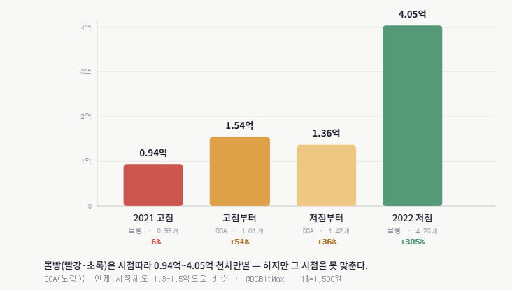
같은 1억, 비트코인 언제 샀느냐로 갈린 결과입니다.
2021 고점에 몰빵 → 4년 반 들고도 −6%
2022 저점에 몰빵 → +305%
딱 1년 차이가 0.94억 vs 4.05억.
근데 그 시점, 누가 미리 맞추나요? 못 맞추니까
— 매일 나눠 사는 DCA(노랑)는 언제 시작해도 1.3~1.5억으로 비슷하게 안착합니다.
그리고 꼭 기억하세요.
저 −6%는 안 팔고 버틴 사람 얘기입니다. 고점에 빚내서 산 사람들은 그 −6%조차 못 누렸어요.
1년 만에 닥친 −77% 구간에서 빚에 떠밀려 바닥에 팔고 나갔으니까요.
고점에 빚투, 빨간 막대보다 더 아래가 현실이었습니다.
Three failed launches.
Tesla weeks from bankruptcy.
Divorce. Press calling him a fraud.
2008 Elon had every reason to quit.
Instead he sat in the wreckage and studied every fragment.
The fourth launch reached orbit.
The power-law model just put #Bitcoin in the bottom 4% of all historical readings
Bottom. Four. Percent.
Deep undervalued territory by every long-term metric
Zoom out. Breathe. Stack
스페이스엑스 상장 그리고 지변님
역사상 초대형 IPO들은 대체로 시장의 낙관론과 광기가 극에 달했을 때 등장했습니다.
사람들이 어떤 가격이든 기꺼이 지불하려 할 때 주식 시장 꼭대기 근처에 있다는 또 하나의 신호라고 생각합니다.
스페이스엑스 주식을 사려고 대출을 받겠다는 사람들을 봤고, 투자 경험이 전혀 없는 사람들까지 스페이스엑스 이야기하는 것을 들었습니다.
스페이스엑스의 상장 가격은 1년전보다 이미 6배나 오른 상태인데 오늘도 20%나 올랐고 엑스의 여러 투자자들은 일론에게 고맙다며 스페이스엑스 주식을 매도하고 있습니다.
그리고 지변님, 엑스를 떠나신다니 아쉽습니다. 아래 그래프에 회색으로 음영 처리된 구간은 미국 경기침체 시기입니다. 새로 회색 구간이 나타날때 웃으며 했제하며 다시 돌아오시면 좋겠습니다. 기다리겠습니다.
Korea’s export data for the first 10 days of the month was absolutely absurd, trending close to 90% YoY.
On historical correlations, that would imply a fair value for the semiconductor index that is potentially 50 to 60% higher than current levels.
Yes, I said that.
World’s first trillionaire was born 6/28/1971. Achieved that trillion June 2026.
Nixon cut all links to gold and put us on a pure fiat standard 1.5 months later on 8/15/1971, making trillionaires possible.
And M2 doubling each decade.
The total US M2 money supply was less than a trillion in 1971.
So from 1971 to 2026:
{22.8/0.71} ~ 32
M2 has increased by 32×
There should be a true scientifically precise monetary standard.
Bitcoin is just that.
BREAKING: SpaceX stock, $SPCX, surges over +30% to a fresh record high and hits $2.3 trillion in market cap.
SpaceX is now the 6th largest public company in the world.
WATCH: South Korean memory chipmaker SK Hynix is looking to choose the Nasdaq for its planned US listing, two sources familiar with the matter told Reuters, opting for the technology-heavy bourse to capitalize on investor appetite for AI-linked stocks https://t.co/MKUNcn0AL0
Bitcoin Noise Model:
Separating Slow Cyclical Drift from True Daily Noise
In price space, slow cyclic drift and daily noise are entangled. Any volatility estimate inevitably averages over a moving offset.
What you get are messy mixture distributions, where cyclic behaviour or regime changes overlap.
This looks different in the space of daily exponents.
There we see:
🔸 cleaner distribution functions, well approximated either by Student-t (already shown by @Giovann35084111) or by Laplace distributions
https://t.co/492RfyUDWI
🔸a relatively stable mean μ(t), slightly different from cycle to cycle
🔸strong but slow intra-cyclical drift, which is essentially is the signal
https://t.co/6LIoM1vddu
https://t.co/KdYNuPxKGO
🔸enormous additional daily stochastic noise, superimposed on that, with max. exponents up to ±1000 or more
This last point makes clear why a cycle mean of n around 6 is so meaningful despite the huge daily noise.
In short: with the daily exponents, we have probably found a clean observable of Bitcoin. On top of that, we can test the stability of the noise model assumptions, Laplace vs Student-t, after applying them to the price space.
The idea is simple: model the price as a Power Law with μ(t) as the exponent and add the noise whose "shape" we already know from the fits in the exponent-space.
We can use a Monte Carlo simulation with a 1-day horizon and determine the width of all simulated paths.
This reveals the daily noise band, as cleanly separated as possible from local bubbles, crashes or wild market regimes!
The interesting part is that noise acts multiplicatively in price space, so it also depends on the absolute price level.
As price anchor, a smoothed price curve can be used and the simulated noise band can be drawn around it. The noise width is therefore automatically adapted both to the current price level and to the distribution width of the current cycle.
Decoupling from the price level also is easy: the noise band is drawn around a theoretical Power-Law Mean instead of the current price.
There are more interesting things one can do. With conventional methods, it is almost impossible to determine the evolution of noise or extrapolate it precisely. With this approach, we can even theoretically determine the function by which future noise should evolve.
Results:
🔸daily noise level decay ~1/t relative to the price level, currently around 7%, will be ~6.5% 04/2028
🔸absolute noise levels will rise, since PL rises: from currently ±8k to ±15k within the next 2 years
Fig1: Q99.9% since 2013, log-log-chart
Fig2: Q99.0% since 2017, linear chart
Fig3: rel. and abs. noise level evolution and extrapolation. Since the '13-cycle noise level was a bit lower, a global fit was not possible, but since halving 2 we see nearly identical levels (semi-global fit in red).
Remarks:
n: exponent of a power law y~t^n
µ: the mean of value of a probability distribution
So if µ is a fit parameter of a probability distribution, it is refered to as µ and not n.