O k a n D e r i n

Assoc. Prof. Dr. of Infectious Diseases & CM Şişli Etfal |

Ph.D. candidate in Epidemiology Medipol Univ. |

#HIV #Rstats #ClimateCrisis #LaiklikKorur

[Joachim Schork @JoachimSchork]

Homoscedasticity is one of those statistical concepts that sounds intimidating at first, but a clear explanation can make it much easier to understand. Breaking down foundational ideas like this helps make data analysis more accessible and strengthens our understanding of statistical models.

Thank you for sharing this, @JuanluCaba_Unex.

#DataScience #Statistics #MachineLearning #DataAnalysis

[O k a n D e r i n @drokanderin]

Prof. Dr. Osman Erol Hayran'ın vefatıyla çok değerli bir hocamızı kaybettik. Bize halk sağlığı ve epidemiyoloji anlatırken vizyon sahibi olmayı, sorgulamayı ve her koşulda erdemli kalabilmeyi de öğretti. Kendisini saygı, minnet ve rahmetle anıyorum. Mekânı cennet olsun.

[Recep Öztürk @DrRecepOzturk]

Ömrünü halk sağlığı ve epidemiyolojiye vakfeden; dekanlık başta olmak üzere üstlendiği muhtelif idari görevleri liyakatle yürüten; binlerce hekim, sağlık çalışanı ve yüzlerce bilim insanı yetiştiren "hocaların hocası" Prof. Dr. Osman Hayran dâr-ı bekâya irtihal etmiştir.

Hacettepe’den Medipol’e uzanan köklü ve müstesna ilim yolculuğunda o, tıbbı salt bir bilgi ve teknik beceriye indirgememiştir. Hekimlik mesleğine daima insanı, toplumu ve vicdanı merkeze alan bir irfan nazarıyla yaklaşmıştır. İnsanın nesneleştiği, şifanın ise ticari bir metaya dönüştüğü bu asırda; "hayatın tıplaştırılması" ve "tıbbın metalaştırılması" tehlikesine karşı her daim haysiyetli bir duruş sergilemiştir. Makaleleri, eserleri ve klinikten kürsüye taşıdığı hakikat arayışıyla, hekimlik sanatının onurunu muhafaza etme yolunda geride sönmeyecek bir meşale bırakmıştır.

Sağlıkta adaleti, hakkaniyeti ve hekimlik erdemini şiar edinen aziz hocamıza Allah’tan rahmet; kederli ailesine, talebelerine ve tüm tıp camiasına sabır ve başsağlığı dilerim.

[KLİMİK Derneği @klimik_dernegi]

Bangladeş'teki Kızamık Salgınında Mart Ortasından Bu Yana Toplam Vaka Sayısı 50 000'i Aştı

Haber İçin: https://t.co/e06hsdG4ga

[KLİMİK Derneği @klimik_dernegi]

KLİMİK Derneği Zoonotik İnfeksiyonlar Çalışma Grubu (ZİÇG) Hantavirus Bilgi Notu 📌

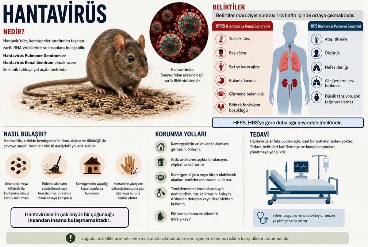
Hantaviruslar, kemiriciler aracılığıyla bulaşan ve ciddi klinik tablolara yol açabilen zoonotik infeksiyon etkenleridir.

İnfekte kemiricilerin idrar, dışkı ve salyası ile kontamine aerosol partiküllerinin solunması en önemli bulaşma yoludur. Hantavirus infeksiyonları başlıca iki önemli klinik tabloya neden olabilir:
▪️Hantavirus Pulmoner Sendromu (HPS) → hızlı gelişen solunum yetmezliği, öksürük, nefes darlığı ve ciddi akciğer tutulumu ile seyredebilir.
▪️Hemorajik Ateş ile Seyreden Renal Sendrom (HFRS) → ateş, hipotansiyon, trombositopeni, kanama bulguları ve akut böbrek yetmezliği ile karakterizedir.

Hastalık çoğu zaman; ateş, halsizlik, kas ağrısı, baş ağrısı, bulantı-kusma gibi nonspesifik belirtilerle başlar ve klinik tablo kısa sürede ağırlaşabilir.

Korunmada;
▪️Kemirici teması ve yaşam alanlarının kontrolü
▪️Kapalı alanların temizlenmeden önce havalandırılması
▪️Temizlik sırasında maske ve eldiven kullanılması önem taşır.
▪️Erken tanı, yakın klinik takip ve uygun destek tedavisi mortalitenin azaltılmasında kritik öneme sahiptir.

🔗https://t.co/5U1I2XmFx7

[TTB-UDEK @TtbUdek]

Hantavirus Bilgi Notu

Ne oldu?

Mayıs 2026’nın ilk günlerinde, Güney Amerika’dan Avrupa’ya doğru seyreden MV Hondius adlı yolcu gemisinde; ateş, gastrointestinal yakınmalar ve hızla ilerleyen solunum yetmezliği ile karakterize bir hastalık kümesi bildirildi. İlk değerlendirmelerde bazı olgularda hantavirüs enfeksiyonu saptandı ve olayın özellikle Andes virüsü ile ilişkili olabileceği belirtildi. Bu durum, hantavirüslerin çoğunlukla kemirgen kaynaklı bulaşan zoonotik etkenler olmasına karşın, Andes virüsü için sınırlı kişiden kişiye bulaşın tanımlanmış olması nedeniyle uluslararası halk sağlığı açısından dikkat çekti.

Bu olay, kamuoyunda “Yeni bir salgın mı söz konusu?”, “Hantavirüs kişiden kişiye bulaşır mı?”, “Türkiye için risk var mı?” gibi soruları gündeme getirdi. Mevcut bilimsel bilgiler, hantavirüs enfeksiyonlarının dünya genelinde nadir görüldüğünü ve bulaşın çoğunlukla enfekte kemirgenlerin idrar, dışkı veya tükürüğüyle kontamine materyallerin solunması yoluyla gerçekleştiğini göstermektedir. Bununla birlikte, Hantavirüs ailesinden Güney Amerika kökenli Andes virüsünün, yakın ve uzun süreli temasla insandan insana bulaştığı belgelenmiştir.

Bu nedenle MV Hondius olayı, geniş toplum için yüksek riskli bir pandemi tehdidi olarak değil; seyahat öyküsü, kemirgen maruziyeti, yakın temaslı izlemi ve erken klinik tanı açısından dikkatle yönetilmesi gereken sınırlı bir halk sağlığı olayı olarak değerlendirilmelidir.

Hantavirüsler küresel ölçekte nadir, ancak ağır seyirli olabilen zoonotik enfeksiyonlardır. Türkiye’de de özellikle Karadeniz bölgesiyle ilişkili daha önce bildirilmiş olgular nedeniyle, ateş, trombositopeni, akut böbrek hasarı veya solunum yetmezliği ile başvuran ve uygun epidemiyolojik öyküsü bulunan hastalarda ayırıcı tanıda akılda tutulmalıdır.

Mayıs 2026’daki MV Hondius olayı, hantavirüslerin temel olarak kemirgen kaynaklı bulaştığını; ancak Andes virüsü gibi özel türlerde sınırlı kişiden kişiye bulaş olasılığının halk sağlığı açısından dikkatle ele alınması gerektiğini göstermektedir.

Bu çerçevede, hantavirüs enfeksiyonuna ilişkin temel bilgiler ve güncel gelişmeler, bilimsel, kısa ve güncel bir soru-cevap formatında özetlenmiştir.

SORULAR ve YANITLAR

1. Hantavirüsler hangi virüs grubudur ve temel rezervuarı nedir?

Hantavirüsler, Hantaviridaeailesinde yer alan, doğal rezervuarı çoğunlukla kemirgenler olan zoonotik RNA virüsleridir. İnsan enfeksiyonu çoğunlukla enfekte kemirgenlerin idrar, dışkı veya tükürüğü ile kontamine materyalin aerosolize olup solunmasıyla gelişir. Korunmanın temelinde insan-kemirgen temasının azaltılması yer alır.
Andes virüsü — ANDV, hantavirüsler içinde özel öneme sahip bir türdür. Güney Amerika’da, özellikle Arjantin ve Şili’de görülen bu virüs, hantavirüs kardiyopulmoner sendromuna — HCPS/HPS neden olabilir. Andes virüsünün temel rezervuarı da kemirgenlerdir; ancak diğer hantavirüslerden farklı olarak, yakın ve uzun süreli temasla sınırlı kişiden kişiye bulaşın kanıtlanmış olduğu başlıca hantavirüs türüdür.

2. Hantavirüs enfeksiyonu dünyada hangi klinik sendromlarla seyreder?

Coğrafi dağılıma göre iki ana klinik tablo vardır. Amerika kıtasında daha çok hantavirüs kardiyopulmoner sendromu — HCPS/HPS görülür; bu tablo akciğer ve kardiyovasküler sistemi etkiler. Avrupa ve Asya’da ise daha çok böbrek sendromlu hemorajik ateş — HFRS görülür; bu tabloda ateş, trombositopeni, kanama eğilimi ve akut böbrek hasarı ön plandadır.

3. Dünya genelinde hastalık yükü ve fatalite nasıldır?

Hantavirüs enfeksiyonları küresel olarak nadir kabul edilmekle birlikte ağır seyredebilir. DSÖ’ye göre dünyada yılda yaklaşık 10.000 ile 100.000’den fazla enfeksiyon geliştiği tahmin edilmektedir. Fatalite, Asya ve Avrupa’daki HFRS tablolarında genellikle %1–15, Amerika kıtasındaki HCPS tablolarında ise %20–40düzeylerine, bazı ağır serilerde %50’yekadar çıkabilir.

4. Hantavirüs kişiden kişiye bulaşır mı?

Genel kural olarak hantavirüsler kişiden kişiye kolay bulaşmaz; insan çoğu zaman “son konak”tır. Ancak Andes virüsü önemli istisnadır. Güney Amerika’da, özellikle Arjantin ve Şili ile ilişkili Andes virüsü enfeksiyonlarında, yakın ve uzun süreli temasla sınırlı kişiden kişiye bulaş gösterilmiştir. Avrupa ve Asya’da görülen Puumala ve Dobrava gibi hantavirüslerde insandan insana bulaş gösterilmemiştir.

5. Klinik olarak hangi hastalarda hantavirüs düşünülmelidir?

Ateş, miyalji, baş ağrısı, gastrointestinal semptomlar, trombositopeni, akut böbrek hasarı veya hızla gelişen dispne/ARDS tablosu olan hastalarda; özellikle kemirgen teması, kırsal alan, depo/ahır/yazlık temizliği, orman-tarla maruziyeti veya endemik bölge seyahati varsa hantavirüs enfeksiyonu ayırıcı tanıda düşünülmelidir. Erken dönem bulguları influenza, COVID-19, leptospiroz, viral pnömoni, sepsis ve diğer viral hemorajik ateşlerle karışabilir.

6. Tanı ve tedavi yaklaşımı nasıldır?

Tanıda seroloji ve moleküler yöntemler kullanılır. Akut enfeksiyonda hantavirüse özgü IgM, serokonversiyon veya artan IgG titreleri gösterilebilir; erken dönemde RT-PCR ile viral RNA saptanabilir. Spesifik ruhsatlı antiviral tedavi veya yaygın kullanıma girmiş aşı yoktur. Tedavinin temelini erken tanı, destek tedavisi, solunum-kardiyak-böbrek komplikasyonlarının izlenmesi ve gerekli olgularda yoğun bakım desteği oluşturur.

7. Türkiye’de hantavirüs enfeksiyonu açısından bilinen durum nedir?

Türkiye’de ilk klinik ve serolojik olarak doğrulanmış hantavirüs salgını 2009’da Zonguldak–Bartın bölgesinde görülmüş; 12 laboratuvar doğrulanmış olgu bildirilmiştir. 2010’da aynı bölgede 8 doğrulanmış olgu ve 1 ölüm daha raporlanmıştır.

Türkiye’de 2009–2025 yılları arasında toplam 336 hantavirüs enfeksiyonu olgusu ve 15 ölüm bildirilmiştir.
8. Mayıs 2026’daki MV Hondius gemi olayı nedir?
DSÖ’ye 2 Mayıs 2026’da, MV Hondius adlı yolcu gemisinde ağır solunum yolu hastalığı kümesi bildirilmiştir. DSÖ’nün 4 Mayıs 2026 güncellemesine göre gemide 7 olgu saptanmış; bunların 2’si laboratuvar doğrulanmış, 5’i şüpheli olarak değerlendirilmiş ve 3 ölümbildirilmiştir. Klinik tablo ateş, gastrointestinal semptomlar, pnömoniye hızlı ilerleme, ARDS ve şok ile karakterizedir.

9. Gemi olayında neden Andes virüsü özellikle önemlidir?

ECDC’nin (Avrupa Enfeksiyon Hastalıkları Kontrolü Merkezi) 6 Mayıs 2026 değerlendirmesine göre gemideki bazı örneklerde hantavirüs PCR pozitifliği saptanmış ve en az bir örnekte Andes virüsü — ANDV doğrulanmıştır. Andes virüsü Güney Amerika’da endemiktir ve kişiden kişiye bulaşın nadiren de olsa belgelenmiş olduğu hantavirüs türüdür. ECDC’nin hipotezine göre bazı yolcuların Arjantin’de maruz kalmış olması ve gemi ortamında yakın temas nedeniyle sınırlı bulaş olasılığı araştırılmaktadır.

10. Bu gemi olayı genel toplum için büyük bir salgın riski anlamına gelir mi?

Mevcut değerlendirmeye göre hayır. DSÖ olayla ilişkili küresel riski düşük, ECDC ise Avrupa genel nüfusu için riski çok düşük olarak değerlendirmiştir. Bunun nedeni, Andes virüsünün kişiden kişiye kolay bulaşmaması, bulaşın genellikle yakın ve uzun süreli temas gerektirmesi ve Andes virüsünün doğal kemirgen rezervuarının Avrupa’da bulunmamasıdır.
Bununla birlikte gemideki yolcular/personel yakın temaslı kabul edilmekte; izolasyon, temaslı izlemi, test, tıbbi takip ve uygun enfeksiyon kontrol önlemleri uygulanmaktadır.

👇
https://t.co/3aUyR5WFH2 @ttborgtr

[O k a n D e r i n @drokanderin]

@RichardDawkins Even if we could bring Neanderthals back, would we treat them with dignity?
History suggests we struggle with anyone who is different.

[Joachim Schork @JoachimSchork]

Speed up data analysis in R with the package suite fastverse. It unites several high-performance R packages for fast data manipulation, transformation, and computation, helping you build efficient workflows with minimal dependencies.

Perfect for:
✔️ Working with large or complex datasets that require speed and efficiency
✔️ Creating lightweight, performance-oriented R pipelines
✔️ Managing a custom collection of optimized R packages in one place
✔️ Projects where compiled code performance (C/C++) makes a real difference

Learn more on GitHub: https://t.co/KLNkSYwAoY

For more on statistics, data science, R, and Python, subscribe to my newsletter. Take a look here for more details: https://t.co/ktUcWo9XpO

#Rpackage #coding #R #database #Data #RStats #datascienceenthusiast

[Mustafa @oprydai]

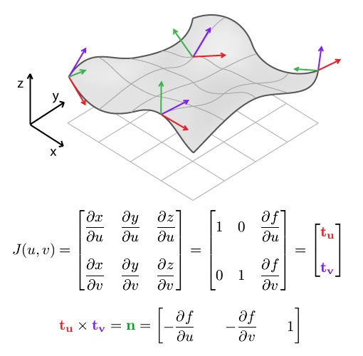
the jacobian matrix is how multivariable systems actually move

you don’t deal with one variable anymore
you deal with transformations

input vector → output vector

the jacobian captures how every input dimension affects every output dimension

what it is:
→ a matrix of partial derivatives
→ each row = one output function
→ each column = one input variable

J(i,j) = ∂f_i / ∂x_j

why it matters:
→ it’s the local linear approximation of a nonlinear system
→ it tells you how small changes propagate
→ it converts messy systems into something you can compute

in physics:
→ coordinate transformations
→ velocity mappings
→ change of variables in integrals

in robotics:
→ maps joint velocities → end-effector velocity
→ singularities show up when the jacobian collapses

in optimization / ML:
→ gradient flow through layers
→ backprop is chained jacobians

interpretation: → determinant ≠ 0 → transformation is locally invertible
→ determinant = 0 → information collapse

the jacobian is not theory
it’s the interface between geometry and computation

[Joachim Schork @JoachimSchork]

Variance estimation is a key part of survey analysis. It helps quantify how much uncertainty is associated with estimates like means or totals. There are many different metrics available, each designed to describe a specific aspect of variability or precision. Using these measures ensures that survey results are interpreted correctly, especially when dealing with complex designs, nonresponse, or weighting.

Here are some key metrics in variance estimation:

1️⃣ Variance: Estimates how much a statistic would vary across repeated samples drawn under the same design
2️⃣ Standard error (SE): The square root of the variance of an estimator; used to construct confidence intervals
3️⃣ Mean squared error (MSE): Combines both variance and bias; useful in model-based or nonrandomized approaches
4️⃣ Margin of error (MoE): Half the width of a confidence interval; indicates the expected range of error
5️⃣ Coefficient of variation (CV): SE divided by the estimate; useful for comparing relative precision across variables or domains
6️⃣ Design effect (Deff): Measures how the sampling design inflates variance compared to simple random sampling

🔹 In R, use the survey or srvyr package to estimate variance while accounting for weights, clustering, stratification, and replicate weights for replication methods.
🔹 In Python, use statsmodels for standard errors and confidence intervals in simple settings, or surveysampling and custom bootstrap/jackknife implementations for more complex survey designs.

For more on statistics, data science, R, and Python, subscribe to my email newsletter. See this link for additional information: https://t.co/ktUcWo9XpO

#Data #datastructure #Rpackage #RStats #Statistical #R

[Matt Dancho (Business Science) @mdancho84]

The Fundamentals Of Building Autonomous LLM Agents

A 38-page PDF that uncovers the secrets of building AI agents that are "agentic"

Get it here:

[Joachim Schork @JoachimSchork]

I've recently published an article titled "Introduction to the R Programming Language – Basic Concepts for Beginners." In this article, I cover fundamental features of R and explain how to use it to manipulate, analyze, and visualize data.

The article was created in collaboration with Tomi Mester, and you can find it on the Data36 website: https://t.co/XqVK7qLSqV

Here’s a glimpse of what you’ll learn:

1️⃣ Background information about the R programming language.
2️⃣ Data manipulation techniques in R.
3️⃣ Calculating descriptive statistics for your data sets.
4️⃣ Creating a correlation matrix to understand variable relationships.
5️⃣ Estimating a linear regression model.
6️⃣ Visualizing data using the ggplot2 package.

You can easily follow along by copying and pasting the R code snippets provided into R or RStudio. Every code example is fully reproducible.

If you're eager to dive deeper into R, check out my course, "Introduction to R Programming for Absolute Beginners." This course is perfect whether you're starting from scratch or looking to refresh your skills.

More information: https://t.co/lUOKp2kv2r

#R4DS #Rpackage #ggplot2 #RStats #DataAnalytics #database

[O k a n D e r i n @drokanderin]

Aesculapius’tan İbn Sina’ya uzanan mirasın ve modern bilimin ışığında hekimliğin sorumluluğunu taşıyoruz. 14 Mart, hem modern tıp eğitiminin başlangıcı hem de bir dayanışma ve mücadele günüdür. Tüm hekimlerin Tıp Bayramı kutlu olsun. #14marttıpbayramıkutluolsun

[Joachim Schork @JoachimSchork]

Effect size measures the strength of a relationship between variables or the difference between groups, providing deeper insights than p-values alone. It helps assess the practical significance of results, making it valuable in fields like psychology, medicine, and social sciences.

✔️ Provides Practical Insight: Quantifies the importance of results beyond statistical significance.
✔️ Enables Comparisons: Allows results to be compared across studies with different scales or sample sizes.
✔️ Supports Meta-Analysis: Useful for combining results from multiple studies.
✔️ Offers Flexibility: Includes measures like Cohen’s d, Hedges’ g, Pearson’s r, and odds ratios for different data types.

❌ Sample Size Sensitivity: Small data sets can produce unstable estimates.
❌ Over-Reliance Risk: Interpreting effect size without confidence intervals can be misleading.
❌ Assumption Sensitivity: Some measures assume normality and equal variance.

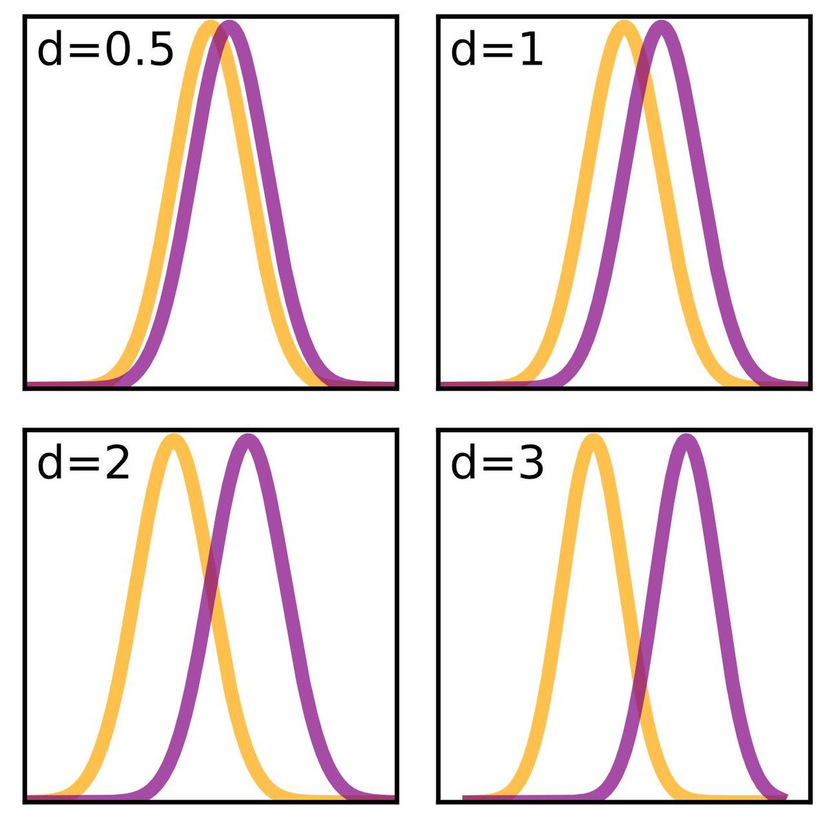
The image below shows plots of Gaussian densities illustrating various values of Cohen's d, highlighting how larger values indicate greater differences between groups. Image credit to Wikipedia: https://t.co/gXrrBbvMSj

🔹 In R: The effectsize package calculates Cohen’s d, Hedges’ g, and other measures, while the MBESS package provides confidence intervals.
🔹 In Python: The statsmodels library offers tools for effect size calculations, and the pingouin library provides user-friendly functions for a range of measures.

Looking to learn more about Statistics, Data Science, R, and Python? Subscribe to my email newsletter! See this link for additional information: https://t.co/ktUcWo9XpO

#Python #Statistical #datastructure #R #RStats

[Joachim Schork @JoachimSchork]

Choosing between R and Python for statistical analysis involves understanding their specific strengths and popularity in different contexts. Python is a versatile programming language, widely favored for its general-purpose capabilities and extensive use in data science and software development. In contrast, R has a strong foothold in the field of statistics, providing specialized tools and packages designed for statistical computing and graphics.

The visualization of this post illustrates Google search trends over the last five years, comparing interest in R and Python for programming and statistics. It shows that while Python generally maintains higher search interest overall, R leads when focusing on statistical topics.

Here’s a comparison of both languages for statistical tasks:

R:

🔹 Highly specialized in statistical analysis and data visualization.
🔹 Offers a wide range of packages specifically for statistical tests, modeling, and graphics (e.g., dplyr, ggplot2, stats).
🔹 Preferred for academic and research-focused projects in statistics.

Python:

🔹 Known for its versatility in data science and general-purpose programming.
🔹 Integrates well with other technologies and supports a broader range of applications, from machine learning to web development.
🔹 Utilizes powerful libraries for data manipulation and visualization (e.g., pandas, matplotlib, seaborn, scipy, statsmodels).

Generally speaking, the choice between R and Python often comes down to personal preference. Both languages have their unique strengths and can be effective for statistical tasks. However, it's also important to consider the ability to communicate and collaborate with peers. In the field of statistics, R is widely used and recognized, making it a valuable tool for ensuring clear communication and understanding within teams. For this reason, I would always choose R for statistical tasks.

If you want to dive deeper into statistical methods in R, check out my online course. Learn more by visiting this link: https://t.co/7YQCRDKSPO

#programmer #Python #Data #VisualAnalytics #DataAnalytics #DataViz

[Joachim Schork @JoachimSchork]

Understanding degrees of freedom (DoF) is crucial because it plays a vital role in determining the accuracy and reliability of various statistical tests. Essentially, DoF refers to the number of independent values or quantities that can vary in a calculation while still meeting certain constraints. In simpler terms, it represents the number of independent pieces of information available to estimate a parameter or test a hypothesis. This concept is critical because it directly shapes the statistical distributions used in tests, which in turn affects the interpretation of results.

Example:

In a simple t-test comparing the means of two groups, the degrees of freedom are determined by the sample size of each group. Specifically, the DoF is calculated as the total number of observations across both groups minus the number of groups being compared (n₁ + n₂ - 2). This value influences the shape of the t-distribution used to determine the p-value, which in turn affects whether the difference between the group means is statistically significant. Without correctly accounting for the DoF, the test could yield inaccurate conclusions.

Key Areas Where Degrees of Freedom (DoF) Matter:

✔️ ANOVA (Analysis of Variance): DoF is crucial for comparing means across multiple groups.
✔️ t-tests: Properly applying DoF ensures accurate comparisons between two groups.
✔️ Chi-square tests: DoF helps determine the significance of relationships between categorical variables.
✔️ Regression analysis: DoF is used to assess the fit and complexity of the model, preventing overfitting.

To Implement DoF Correctly in Practice:

🔹 R: Functions like t.test() and chisq.test() automatically calculate the correct degrees of freedom from the data. For custom applications (e.g., simulations or plotting), you can manually specify the DoF using distribution functions like dt() or dchisq().
🔹 Python: Leverage the scipy.stats module, particularly functions like chi2 and t, where the DoF parameter (df) must be correctly defined.

The visualization provided shows chi-square distributions for various degrees of freedom (k = 1, 2, 3, 4, 6, 9). It illustrates how the distribution shape changes with different DoF values, highlighting the importance of selecting the appropriate DoF in your analysis. This visualization is based on one originally from Wikipedia: https://t.co/E5TQyH8QJD

You might check out my online course on Statistical Methods in R, where this topic and others are explained in further detail. Take a look here for more details: https://t.co/7YQCRDKSPO

#RStats #statisticsclass #Python #statisticians #Python3

[Joachim Schork @JoachimSchork]

Multicollinearity is a common issue in regression analysis where predictor variables are highly correlated, leading to unreliable estimates of regression coefficients.

Understanding and addressing multicollinearity is crucial for accurate and reliable statistical modeling.

Challenges of Ignoring Multicollinearity:
❌ Unreliable Coefficient Estimates: Ignoring multicollinearity can result in inflated standard errors and unreliable estimates, making it difficult to determine the true effect of each predictor.
❌ Misleading Interpretations: High multicollinearity can lead to misinterpretations of the significance of predictors, potentially leading to incorrect conclusions.

Benefits of Addressing Multicollinearity:
✔️ Improved Model Accuracy: Properly handling multicollinearity ensures that the estimated coefficients reflect the true relationship between predictors and the outcome variable.
✔️ Enhanced Predictive Power: Addressing multicollinearity helps in building models that generalize well to new data, improving prediction quality.

To handle multicollinearity effectively, consider the following approaches in practice:
🔹 R: Use the car package and the vif() function to detect multicollinearity. If necessary, apply principal component analysis (PCA) or remove highly correlated variables.
🔹 Python: Utilize the statsmodels library to check Variance Inflation Factor (VIF) values and consider using dimensionality reduction techniques like PCA from the sklearn library.

In the accompanying visualization, based on an image from Wikipedia (link: https://t.co/lWcDlwEJN2), the true parameters are reliably estimated when predictors are uncorrelated (black case), but estimation becomes unreliable when predictors are correlated (red case).

To explain this topic in further detail, I collaborated with Micha Gengenbach to create a comprehensive tutorial: https://t.co/9B6Aaxj9jT

Interested in gaining deeper insights into statistics and R programming? Consider joining my online course, "Statistical Methods in R."

Check out this link for more details: https://t.co/7YQCRDKSPO

#datascienceenthusiast #RStats #pythonprogramming #R4DS #Python

[Joachim Schork @JoachimSchork]

Markov chains are a fundamental concept in probability theory, modeling systems that undergo transitions from one state to another in a random process. They rely on the memoryless property, where the future state depends only on the current state, not the past. When properly utilized, Markov chains can unlock powerful insights across various fields, from finance to genetics.

However, improper handling of Markov chains can lead to significant drawbacks.

Challenges of Markov Chains:
❌ Misinterpretation: Without a thorough understanding, results derived from Markov chains might be misleading, particularly if the memoryless property is overlooked.
❌ Data Dependency: Markov chains rely heavily on accurate and representative data. If the data set is not sufficiently robust, the chain’s predictions could be inaccurate.
❌ Complexity: For large systems, constructing a Markov chain becomes increasingly complex, often requiring sophisticated computational tools and techniques.

Benefits of Markov Chains:
✔️ Predictive Modeling: When correctly applied, Markov chains can help forecast future states in a system based on its current state, leading to more accurate predictive models.
✔️ Simplified Analysis: They break down complex systems into manageable parts, allowing for a clearer understanding of each component and its behavior.
✔️ Versatile Applications: Markov chains are highly adaptable, with applications in queueing theory, economics, and machine learning, making them a versatile tool in a data scientist's arsenal.

To implement Markov chains in practice:
🔹 R: Use the markovchain package to create and analyze discrete-time Markov chains, which simplifies transitions, state spaces, and probabilities.
🔹 Python: Utilize the pymc or hmmlearn libraries to model and infer the hidden states in sequential data.

The following visualization, based on a Wikipedia image (link: https://t.co/14n49FraJI), shows a simple two-state Markov process. The numbers represent the probabilities of transitioning from one state to another, illustrating the flow within the system.

To explain this topic in further detail, I collaborated with Micha Gengenbach to create a comprehensive tutorial: https://t.co/bpqZXmvZgp

Want to dive deeper? Enroll in my online course, "Statistical Methods in R." More information: https://t.co/7YQCRDKSPO

#database #RStats #programming #RStudio #Python

[UN News @UN_News_Centre]

#Somalia is facing a rapidly worsening drought after four failed rainy seasons, leaving millions at risk of hunger and displacement, warns @OCHASom.

https://t.co/fulBhA1Ne7

[Joachim Schork @JoachimSchork]

gander is an R package that brings AI directly into RStudio or Posit.

Instead of switching between your IDE and a chat window, gander lets you ask questions or request code changes right inside your script. It automatically shares relevant context such as variable names, data types, and the surrounding code, so the model can provide precise answers without extra copy-pasting.

You can trigger it with a simple keyboard shortcut, choose from different AI models (OpenAI, Claude, or local ones), and control how much of your data is sent for context. In short, gander makes working with AI in RStudio smoother, faster, and smarter.

Take a look at the visualization below. It shows an example of how to use gander to create a ggplot2 graph. It’s taken from the package website: https://t.co/DbsZTbsmVK

Join my newsletter for more tutorials and insights on R, Python, data science, and AI. For more information, visit this link: https://t.co/X93SeCe0rb

#Python #programmer #DataAnalytics #Rpackage #ggplot2 #DataViz #Statistics #RStats #DataVisualization #database #tidyverse #R4DS