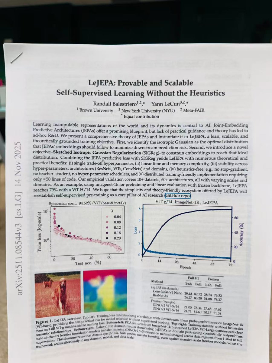
Top Tweets for #LeJEPA
2/ In #LeAVJEPA, we extend #LeJEPA (by @randall_balestr and @ylecun) to audio and video using one shared transformer. During training, 🎤 audio-only and 📹 video-only views learn to match a representation formed from both modalities.
Reading Club discussions on #LeJEPA
🔷 LeJEPA does not require diffusion or reconstruction — that’s the real robot win.
Pure latent predictive coding + distribution matching. Inference is encoder + lightweight predictor → significantly lower latency than diffusion-based world models. No denoising steps or pixel generation, making it compatible with real-time control regimes (e.g. tens-of-Hz robotics loops).
🔷 The framework stays simple by shifting stability into distributional constraints.
It does not rely on stop-gradient, EMA teachers, or other common collapse-prevention heuristics (unlike BYOL-style SSL). A single λ∈[0.1,0.5] suffices, and it remains stable across architectures. For robotics, this yields dense spatial representations usable by downstream policies without generative latency overhead.
🔷 High dimensionality is not a blocker — SIGReg is designed to sidestep it.
The random-projection design sidesteps the curse of dimensionality by operating on low-dimensional slices. With appropriate predictors, unpooled high-resolution features become tractable, enabling strong geometric regularization alongside fine-grained spatial semantics.
🔷 SIGReg never claims full joint isotropic Gaussian — it only pushes projected marginals.
LeJEPA’s SIGReg uses random 1D projections + sketched/MC Epps–Pulley test (a differentiable CF-based normality statistic) to encourage approximate isotropy. It sidesteps explicit high-dim density estimation via Cramér–Wold theorem-type arguments (near-linear O(N·M·K), M≈10–100) and mitigates collapse without guaranteeing a perfectly whitened joint distribution. This is a key reason it remains stable even on unpooled features.
🔷 Pooled LeJEPA feels easy because the predictor is simple — unpooled is not a drop-in.
Original pooled/global vectors (CLS or avg-pool) let a tiny MLP perform well-conditioned one-step regression on clean Gaussian targets. For unpooled ([B,N,D] or [B,H,W,D]), the predictive L2 loss still works but typically requires a spatially-aware predictor (e.g. lightweight cross-attn) to capture token correlations. High H×W makes naive regression substantially harder.
🔷 SIGReg still works on unpooled feats, but you can’t just flatten and ignore token dependence.
Applying SIGReg over flattened tokens (or pooled variants) remains effective with near-linear scaling. However, patch tokens are strongly correlated and non-i.i.d., so naive concatenation can bias effective sample size or allow spatial degeneracy. Practical setups often add structure-aware handling (e.g., per-token normalization or mixed pooled+unpooled regularization).
![junfanzhu98's tweet photo. Reading Club discussions on #LeJEPA
🔷 LeJEPA does not require diffusion or reconstruction — that’s the real robot win.
Pure latent predictive coding + distribution matching. Inference is encoder + lightweight predictor → significantly lower latency than diffusion-based world models. No denoising steps or pixel generation, making it compatible with real-time control regimes (e.g. tens-of-Hz robotics loops).
🔷 The framework stays simple by shifting stability into distributional constraints.
It does not rely on stop-gradient, EMA teachers, or other common collapse-prevention heuristics (unlike BYOL-style SSL). A single λ∈[0.1,0.5] suffices, and it remains stable across architectures. For robotics, this yields dense spatial representations usable by downstream policies without generative latency overhead.
🔷 High dimensionality is not a blocker — SIGReg is designed to sidestep it.
The random-projection design sidesteps the curse of dimensionality by operating on low-dimensional slices. With appropriate predictors, unpooled high-resolution features become tractable, enabling strong geometric regularization alongside fine-grained spatial semantics.
🔷 SIGReg never claims full joint isotropic Gaussian — it only pushes projected marginals.
LeJEPA’s SIGReg uses random 1D projections + sketched/MC Epps–Pulley test (a differentiable CF-based normality statistic) to encourage approximate isotropy. It sidesteps explicit high-dim density estimation via Cramér–Wold theorem-type arguments (near-linear O(N·M·K), M≈10–100) and mitigates collapse without guaranteeing a perfectly whitened joint distribution. This is a key reason it remains stable even on unpooled features.
🔷 Pooled LeJEPA feels easy because the predictor is simple — unpooled is not a drop-in.
Original pooled/global vectors (CLS or avg-pool) let a tiny MLP perform well-conditioned one-step regression on clean Gaussian targets. For unpooled ([B,N,D] or [B,H,W,D]), the predictive L2 loss still works but typically requires a spatially-aware predictor (e.g. lightweight cross-attn) to capture token correlations. High H×W makes naive regression substantially harder.
🔷 SIGReg still works on unpooled feats, but you can’t just flatten and ignore token dependence.
Applying SIGReg over flattened tokens (or pooled variants) remains effective with near-linear scaling. However, patch tokens are strongly correlated and non-i.i.d., so naive concatenation can bias effective sample size or allow spatial degeneracy. Practical setups often add structure-aware handling (e.g., per-token normalization or mixed pooled+unpooled regularization).](https://pbs.twimg.com/media/HG-O6Yqa8AA-myJ.jpg)
🦤 LeWorldModel: Learning Physics from Pixels — Stable World Models with Just Two Losses
World models:
1️⃣ DINO-WM: pretrained ViT encoder (from ImageNet) → features → predictor. But encoder is frozen, so no end-to-end learning. Its “visual genetics” are tuned for coarse classification (cats vs dogs), not physics: hard to resolve mm-level changes (e.g., 2 mm block motion). A powerful predictor on top of a “myopic” encoder = blind physical reasoning.
2️⃣ PLDM: end-to-end, but unstable and collapse-prone. Rely on reward as prediction target, so it only works in environments with explicit rewards (e.g., games).
3️⃣ JEPA (Joint Embedding Predictive Architecture): predict next latent instead of pixels. Two hard problems:
collapse (encoder → constant vector, e.g., all zeros)
achieving pixel-level + end-to-end + stable jointly
💡 LeWM solves:
👉 JEPA that trains stably end-to-end from raw pixels
👉 Single hyperparameter λ:
next-embedding prediction
SIGReg (Gaussian regularization)
🧠 #1: true end-to-end
No frozen encoder. Perception + dynamics co-evolve → representation aligned with fine-grained physics, not ImageNet bias.
🧠 #2: “only” one hyperparameter
PLDM needs ~6. LeWM needs 1 (λ) → weight of SIGReg. Plug-and-play, stable.
⚠️ Collapse problem
Encoder could map all inputs → same vector → trivial prediction → zero loss → useless model.
🧩 SIGReg (Gaussian Integral Signature Regularization)
Core: prevent collapse via distribution constraints.
Sample 1024 random directions
Project embeddings → 1024 1D “shadows”
Each must pass Epps–Pulley test (≈ standard normal)
Loss pushes test statistic → 0
Any failed projection ⇒ penalty
Why it works:
Cramér–Wold theorem → a high-dim distribution is determined by its 1D projections.
👉 Enforcing Gaussianity across 1D projections precludes degenerate collapse under projection constraints
🧪 Physical probing
Train in PushT (push block to target), then:
Linear probe recovers: block position, angle, end-effector
👉 physics is linearly decodable
🚨 Teleport block (physically impossible):
embedding anomaly spikes sharply
👉 model internalizes constraint: objects cannot teleport
👉 not inferred from pixel surface features, but encoded as latent constraints
📈 Temporal straightness
No smoothness loss, yet trajectories in latent space are ~straight lines
👉 no prior, purely from “predict next embedding”
👉 implies physically consistent motion, not blurry interpolation
⚡ Performance
Planning: 0.98s vs 47s (DINO-WM)
Success: 96% vs 78% (PLDM)
Why faster?
DINO-WM: frozen encoder → info loss → extra online passes
LeWM: end-to-end → representation already task-aligned
👉 0.98s = fast to handle dynamic obstacles & real-time control
⚠️ Limitations
~15M params (“ant-scale”) → fails on OGBench-Cube (complex physics)
not yet tested on real robots
🔥LeWM shows:
👉 JEPA + SIGReg = stable world models
👉 raw pixels → physics-aware latent space
👉 minimal design (2 losses, 1 hyperparameter)
Next step: scale + real-world deployment 🤖
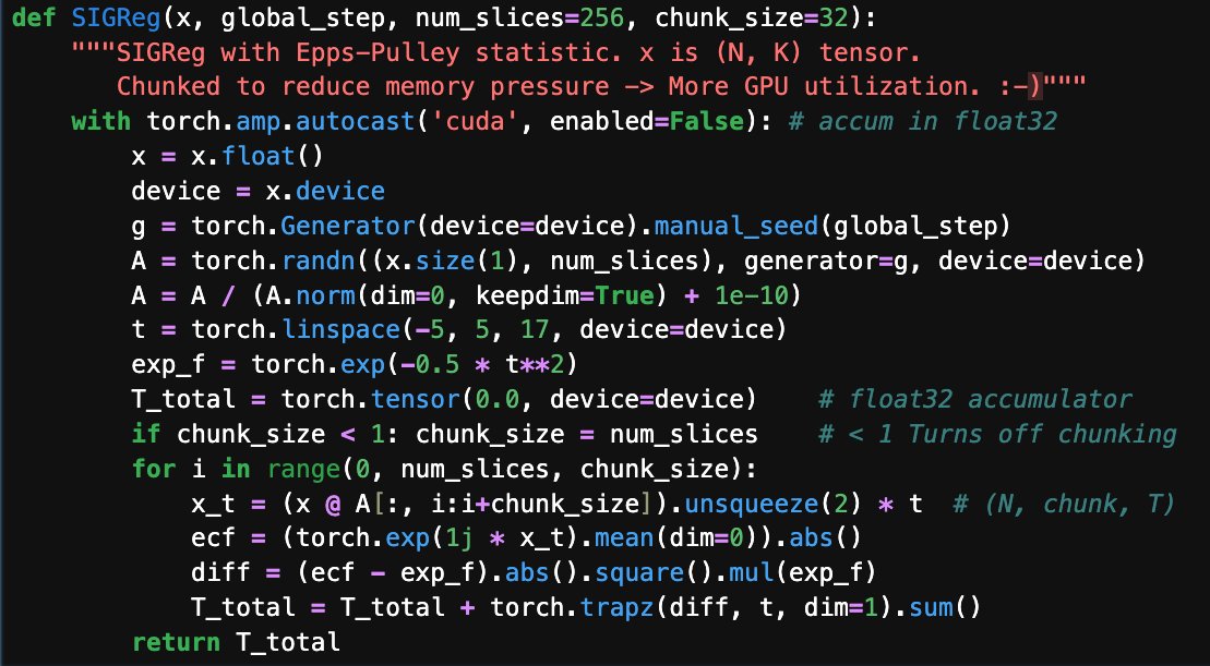
GPU-poor tip for #LeJEPA: chunk your SIGReg slices. 256 slices / chunks of 32 = 8x less VRAM, and it even completes *faster* on my 4090(MaxQ). Giant complex exponential tensors were my bottleneck. One extra loop. Now more room for batch_size! cc @randall_balestr
Last Seen Hashtags on Sotwe
Trends for you
Most Popular Users

Elon Musk 
@elonmusk
241.3M followers

Barack Obama 
@barackobama
118.8M followers

Cristiano Ronaldo 
@cristiano
114.5M followers

Donald J. Trump 
@realdonaldtrump
111.9M followers

Narendra Modi 
@narendramodi
107M followers

Rihanna 
@rihanna
98.7M followers

NASA 
@nasa
92.3M followers

Justin Bieber 
@justinbieber
91.8M followers

KATY PERRY 
@katyperry
90M followers

Taylor Swift 
@taylorswift13
84M followers

Lady Gaga 
@ladygaga
75.5M followers

Virat Kohli 
@imvkohli
73.4M followers

Kim Kardashian 
@kimkardashian
70.8M followers

YouTube 
@youtube
68.7M followers

Neymar Jr 
@neymarjr
66.4M followers

Bill Gates 
@billgates
65.2M followers

Selena Gomez 
@selenagomez
63.1M followers

The Ellen Show
@theellenshow
62.2M followers

CNN 
@cnn
61.7M followers

X 
@x
60.7M followers


![junfanzhu98's tweet photo. Reading Club discussions on #LeJEPA
🔷 LeJEPA does not require diffusion or reconstruction — that’s the real robot win.
Pure latent predictive coding + distribution matching. Inference is encoder + lightweight predictor → significantly lower latency than diffusion-based world models. No denoising steps or pixel generation, making it compatible with real-time control regimes (e.g. tens-of-Hz robotics loops).
🔷 The framework stays simple by shifting stability into distributional constraints.
It does not rely on stop-gradient, EMA teachers, or other common collapse-prevention heuristics (unlike BYOL-style SSL). A single λ∈[0.1,0.5] suffices, and it remains stable across architectures. For robotics, this yields dense spatial representations usable by downstream policies without generative latency overhead.
🔷 High dimensionality is not a blocker — SIGReg is designed to sidestep it.
The random-projection design sidesteps the curse of dimensionality by operating on low-dimensional slices. With appropriate predictors, unpooled high-resolution features become tractable, enabling strong geometric regularization alongside fine-grained spatial semantics.
🔷 SIGReg never claims full joint isotropic Gaussian — it only pushes projected marginals.
LeJEPA’s SIGReg uses random 1D projections + sketched/MC Epps–Pulley test (a differentiable CF-based normality statistic) to encourage approximate isotropy. It sidesteps explicit high-dim density estimation via Cramér–Wold theorem-type arguments (near-linear O(N·M·K), M≈10–100) and mitigates collapse without guaranteeing a perfectly whitened joint distribution. This is a key reason it remains stable even on unpooled features.
🔷 Pooled LeJEPA feels easy because the predictor is simple — unpooled is not a drop-in.
Original pooled/global vectors (CLS or avg-pool) let a tiny MLP perform well-conditioned one-step regression on clean Gaussian targets. For unpooled ([B,N,D] or [B,H,W,D]), the predictive L2 loss still works but typically requires a spatially-aware predictor (e.g. lightweight cross-attn) to capture token correlations. High H×W makes naive regression substantially harder.
🔷 SIGReg still works on unpooled feats, but you can’t just flatten and ignore token dependence.
Applying SIGReg over flattened tokens (or pooled variants) remains effective with near-linear scaling. However, patch tokens are strongly correlated and non-i.i.d., so naive concatenation can bias effective sample size or allow spatial degeneracy. Practical setups often add structure-aware handling (e.g., per-token normalization or mixed pooled+unpooled regularization).](https://pbs.twimg.com/media/HG-O0AzaAAAfJKm.jpg)
![junfanzhu98's tweet photo. Reading Club discussions on #LeJEPA
🔷 LeJEPA does not require diffusion or reconstruction — that’s the real robot win.
Pure latent predictive coding + distribution matching. Inference is encoder + lightweight predictor → significantly lower latency than diffusion-based world models. No denoising steps or pixel generation, making it compatible with real-time control regimes (e.g. tens-of-Hz robotics loops).
🔷 The framework stays simple by shifting stability into distributional constraints.
It does not rely on stop-gradient, EMA teachers, or other common collapse-prevention heuristics (unlike BYOL-style SSL). A single λ∈[0.1,0.5] suffices, and it remains stable across architectures. For robotics, this yields dense spatial representations usable by downstream policies without generative latency overhead.
🔷 High dimensionality is not a blocker — SIGReg is designed to sidestep it.
The random-projection design sidesteps the curse of dimensionality by operating on low-dimensional slices. With appropriate predictors, unpooled high-resolution features become tractable, enabling strong geometric regularization alongside fine-grained spatial semantics.
🔷 SIGReg never claims full joint isotropic Gaussian — it only pushes projected marginals.
LeJEPA’s SIGReg uses random 1D projections + sketched/MC Epps–Pulley test (a differentiable CF-based normality statistic) to encourage approximate isotropy. It sidesteps explicit high-dim density estimation via Cramér–Wold theorem-type arguments (near-linear O(N·M·K), M≈10–100) and mitigates collapse without guaranteeing a perfectly whitened joint distribution. This is a key reason it remains stable even on unpooled features.
🔷 Pooled LeJEPA feels easy because the predictor is simple — unpooled is not a drop-in.
Original pooled/global vectors (CLS or avg-pool) let a tiny MLP perform well-conditioned one-step regression on clean Gaussian targets. For unpooled ([B,N,D] or [B,H,W,D]), the predictive L2 loss still works but typically requires a spatially-aware predictor (e.g. lightweight cross-attn) to capture token correlations. High H×W makes naive regression substantially harder.
🔷 SIGReg still works on unpooled feats, but you can’t just flatten and ignore token dependence.
Applying SIGReg over flattened tokens (or pooled variants) remains effective with near-linear scaling. However, patch tokens are strongly correlated and non-i.i.d., so naive concatenation can bias effective sample size or allow spatial degeneracy. Practical setups often add structure-aware handling (e.g., per-token normalization or mixed pooled+unpooled regularization).](https://pbs.twimg.com/media/HG-OxIda0AAjSPA.jpg)
![junfanzhu98's tweet photo. Reading Club discussions on #LeJEPA
🔷 LeJEPA does not require diffusion or reconstruction — that’s the real robot win.
Pure latent predictive coding + distribution matching. Inference is encoder + lightweight predictor → significantly lower latency than diffusion-based world models. No denoising steps or pixel generation, making it compatible with real-time control regimes (e.g. tens-of-Hz robotics loops).
🔷 The framework stays simple by shifting stability into distributional constraints.
It does not rely on stop-gradient, EMA teachers, or other common collapse-prevention heuristics (unlike BYOL-style SSL). A single λ∈[0.1,0.5] suffices, and it remains stable across architectures. For robotics, this yields dense spatial representations usable by downstream policies without generative latency overhead.
🔷 High dimensionality is not a blocker — SIGReg is designed to sidestep it.
The random-projection design sidesteps the curse of dimensionality by operating on low-dimensional slices. With appropriate predictors, unpooled high-resolution features become tractable, enabling strong geometric regularization alongside fine-grained spatial semantics.
🔷 SIGReg never claims full joint isotropic Gaussian — it only pushes projected marginals.
LeJEPA’s SIGReg uses random 1D projections + sketched/MC Epps–Pulley test (a differentiable CF-based normality statistic) to encourage approximate isotropy. It sidesteps explicit high-dim density estimation via Cramér–Wold theorem-type arguments (near-linear O(N·M·K), M≈10–100) and mitigates collapse without guaranteeing a perfectly whitened joint distribution. This is a key reason it remains stable even on unpooled features.
🔷 Pooled LeJEPA feels easy because the predictor is simple — unpooled is not a drop-in.
Original pooled/global vectors (CLS or avg-pool) let a tiny MLP perform well-conditioned one-step regression on clean Gaussian targets. For unpooled ([B,N,D] or [B,H,W,D]), the predictive L2 loss still works but typically requires a spatially-aware predictor (e.g. lightweight cross-attn) to capture token correlations. High H×W makes naive regression substantially harder.
🔷 SIGReg still works on unpooled feats, but you can’t just flatten and ignore token dependence.
Applying SIGReg over flattened tokens (or pooled variants) remains effective with near-linear scaling. However, patch tokens are strongly correlated and non-i.i.d., so naive concatenation can bias effective sample size or allow spatial degeneracy. Practical setups often add structure-aware handling (e.g., per-token normalization or mixed pooled+unpooled regularization).](https://pbs.twimg.com/media/HG-OsLUbAAABmrV.jpg)