Huzi

thinking about thinking

[Huzi @huzicheng]

Joint work with @zwzhang36 🙌
Paper: Not All Thinking Is Created Equal https://t.co/3GZ8JjjldK
Blog: https://t.co/63RBUYcdI4

[Huzi @huzicheng]

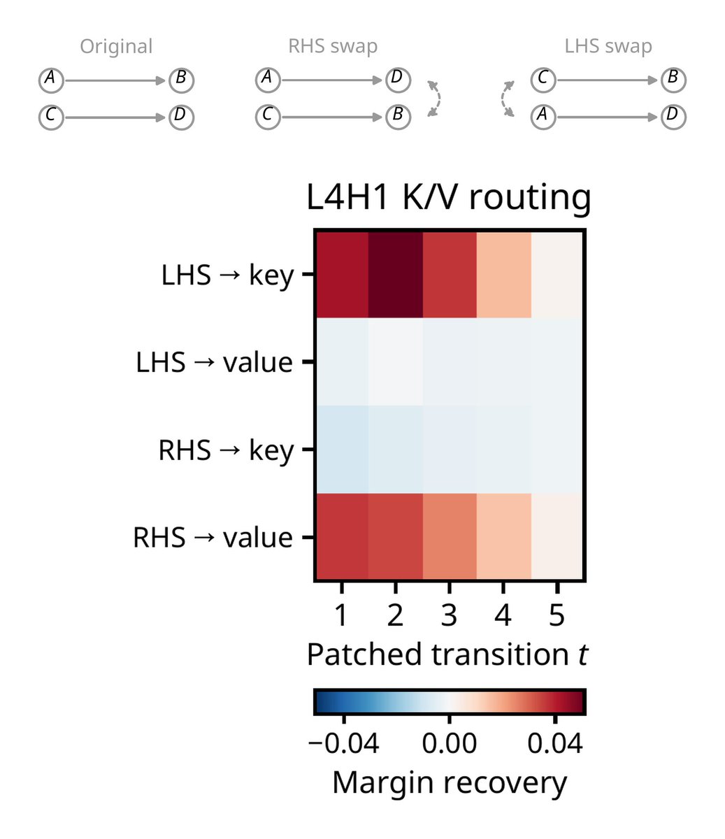
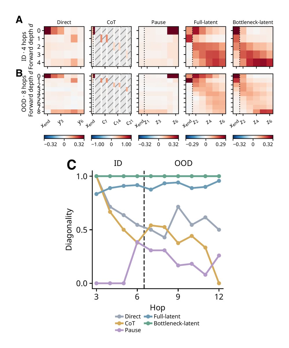
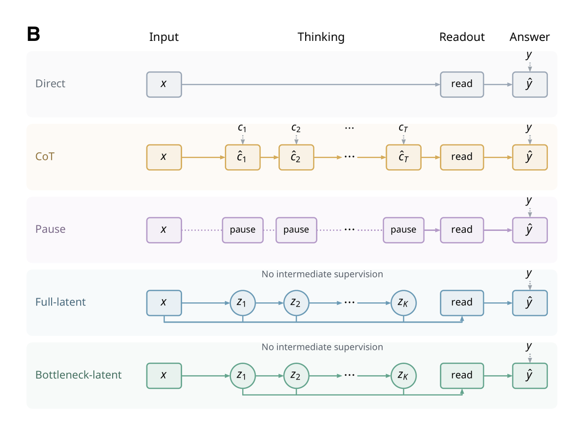
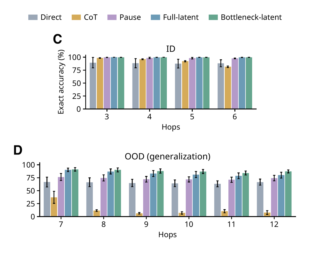
Same in-distribution scores, different algorithms: pause tokens get the same 6 slots minus the loop, yet generalize clearly worse.

Small model, one synthetic task. this is by design, so the circuit could be dissected. Whether large LLMs can do similar stuff is the next question.

[Huzi @huzicheng]

At its core, one attention head follows edges like a lookup table. For "A is B", the key carries A (the address), the value carries B (the content). The thought queries with the nodes it has reached; an MLP + residual stream write the result into the next thought.

[Huzi @huzicheng]

The latent models instead learn forward search, especially the bottleneck one. Their thoughts align with the nodes reachable from the root in d hops (RSA), and the best-matching thought shifts later as d grows, even at unseen depths.

[Huzi @huzicheng]

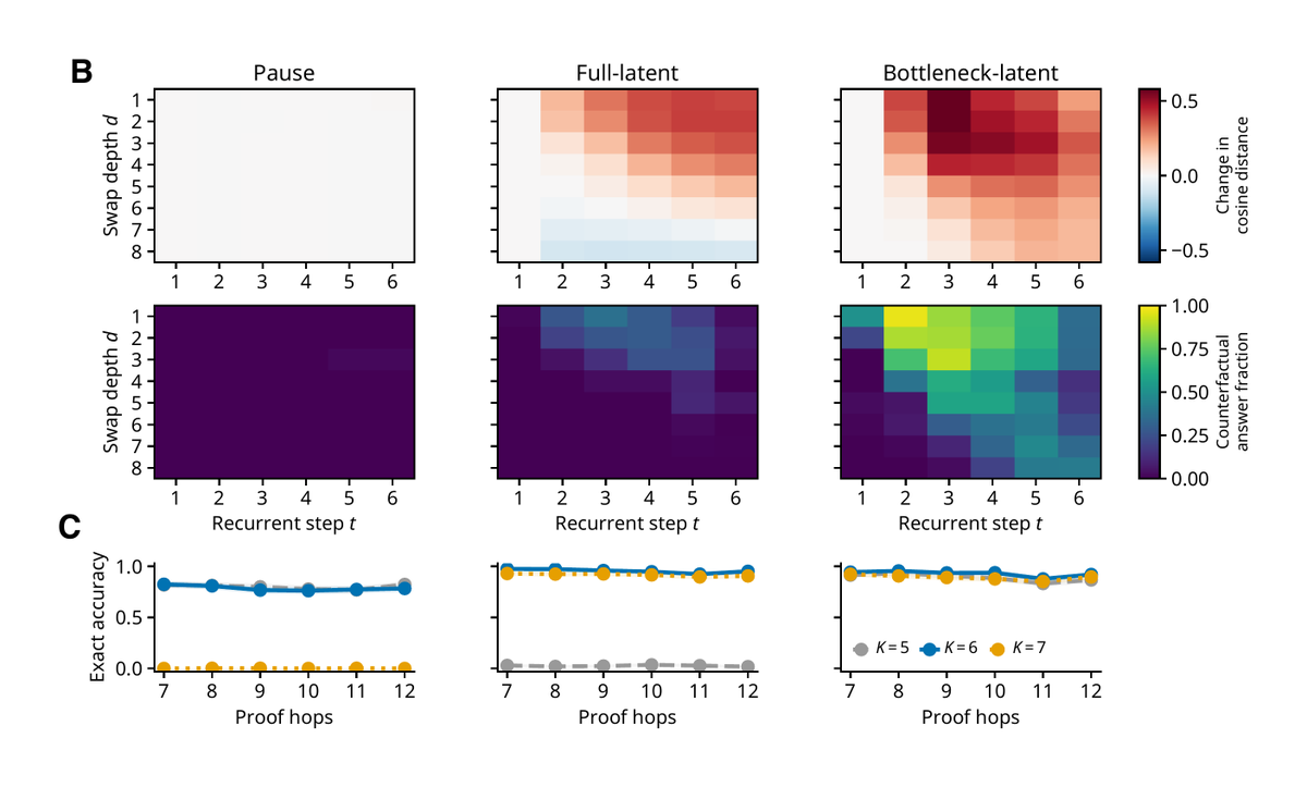
Causal test: swap two edges at depth d to flip the answer, then transplant one thought from the flipped run.

In the bottleneck model, shallow swaps flip the answer from early thoughts, deep ones only from later ones: a for-loop. But a soft one.

[Huzi @huzicheng]

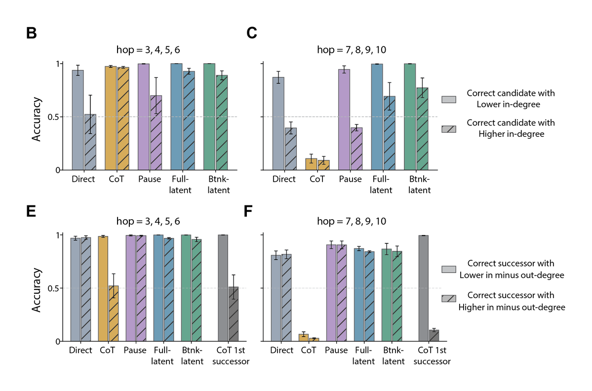
It turns out the others rely on local shortcuts. Direct & pause-token models key on the candidates' in-degree. CoT writes a proof, but its first step follows the degrees of the root's successors; swap those and its step and answer changes too

[Huzi @huzicheng]

The bottleneck variant also drops the prompt at answer time. It can't look back at the question, so everything it knows has to stay inside its 6 thoughts. That's what makes the reasoning inspectable.

[Huzi @huzicheng]

The latent variants feed each step's final hidden state back in as the next input, 6 times. That's Coconut's idea @Ber18791531, but with no curriculum, no reasoning traces, no RL.

[Huzi @huzicheng]

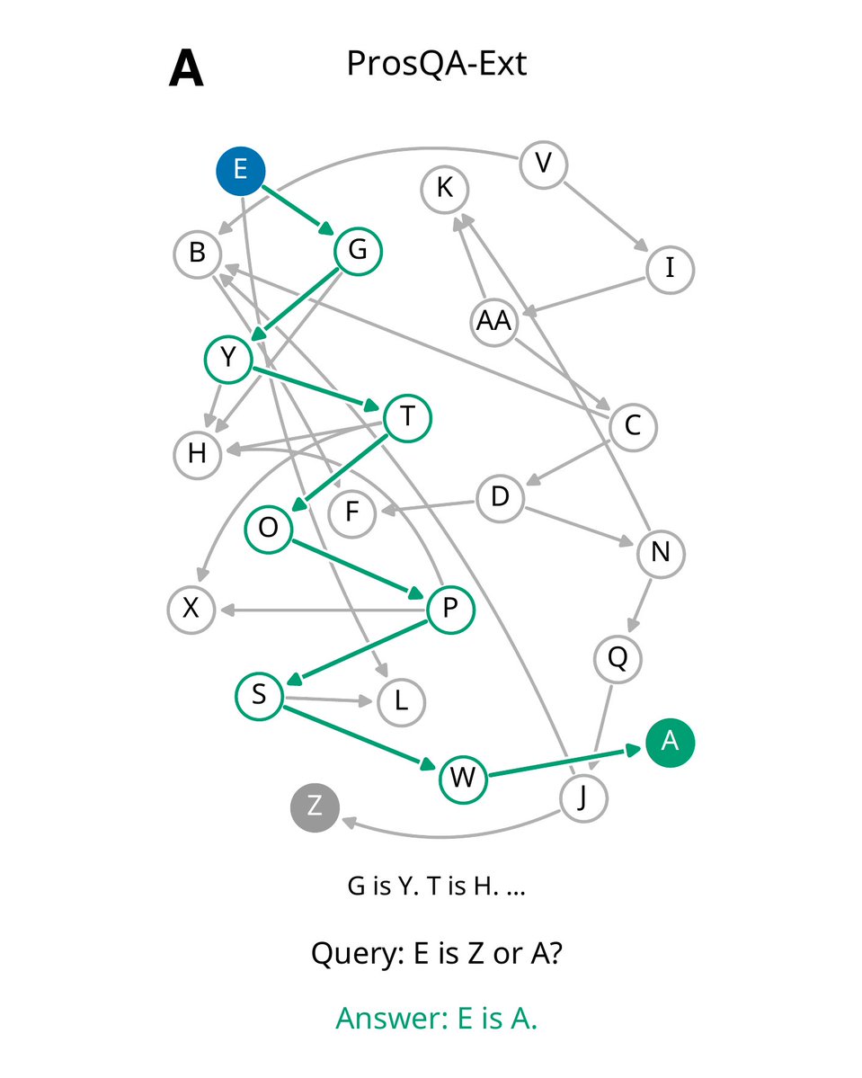
Task: "A is B." premises describe a graph; which of two candidates can the root reach? Train on 3–6 hops, test on 7–12.
Same 4-layer GPTNeoX, from scratch, same data & budget. Only thinking changes: answer directly, write a CoT proof, use pause tokens, or think in latent space.

[Huzi @huzicheng]

Same transformer, five ways to "think." Deeper than anything in training: the variant supervised on step-by-step proofs generalizes worst; the ones trained on Q&A alone, thinking in latent space, generalize best. We traced their algorithm. 🧵

[Jorge Bravo Abad @bravo_abad]

Backprop-free planning: goal-directed sampling from learned cognitive maps

Most planners we deploy today are expensive. RL needs retraining when the goal changes, MCTS and MPC re-search the space at every decision, and all of it usually rides on deep networks and gradient-heavy training. Brains do something different: they plan online, adapt to new goals instantly, and run on about 20 watts. What data structure and learning rule makes that possible?

Hui Lin and coauthors offer a concrete answer. They build a generative cognitive map learner (GCML), a transparent network that learns a forward model plus a linear inverse model through local, Hebbian-style plasticity, so no backpropagation and no backprop through time. The trick for planning is stochastic: they inject Gaussian noise into action selection, which turns a deterministic map-follower into a generative sampler. Given a goal state, the inverse model points roughly toward it, and repeated noisy sampling produces a diverse set of goal-directed trajectories that self-correct back toward the target even after a bad first step.

They validate it in three very different settings from one recipe. In 2D navigation it reproduces rodent hippocampal replay, including rerouting around novel barriers and visiting space never seen during training. On random graphs it becomes an online approximate k-shortest-path solver, returning a menu of near-optimal routes. On an NP-hard tiling task it decomposes shapes it never encountered, trained on 5-block silhouettes and generalizing to 8, with near-perfect success.

The efficiency numbers are the real story for practitioners. Against K*, mA*, BELA*, an RL baseline and MPC, GCML visits far fewer nodes, generates the first step immediately without building a full solution path, and pays essentially zero replanning cost when the goal moves. Because the update rule is local, it maps cleanly onto in-memory and neuromorphic hardware.

This is a template for planning at the edge. In materials screening, drug candidate routing, or energy system control, where goals shift constantly and compute budgets are tight, a model that learns online and replans for free could replace heavy retraining loops with something you can run on-device. It is a reminder that solving genuinely novel problems does not always require a large model.

Paper: Lin et al., Nature Machine Intelligence (2026), CC BY 4.0 | https://t.co/nl1QNE5gIB

[Seohong Park @seohong_park]

What if we represent a state as a "list" of similarities to all other states? In our recent ICLR paper, we studied this "dual" representation.

Come visit our poster at #4608 10:30a-1p on Fri (morning, 2nd day)!

Paper: https://t.co/zYKFjyO0i4
Blog post: https://t.co/lw1Port5k6

[Ching-Lung Hsu @hiallen72]

https://t.co/OnRBihqgTA

[Boris Cherny @bcherny]

I'm Boris and I created Claude Code. Lots of people have asked how I use Claude Code, so I wanted to show off my setup a bit.

My setup might be surprisingly vanilla! Claude Code works great out of the box, so I personally don't customize it much. There is no one correct way to use Claude Code: we intentionally build it in a way that you can use it, customize it, and hack it however you like. Each person on the Claude Code team uses it very differently.

So, here goes.

[Jorge Bravo Abad @bravo_abad]

Fundamental limits of reservoir computing: stability vs. reach

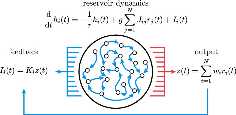
Reservoir computing (RC) uses the natural dynamics of a large recurrent network to generate time-varying signals. You only train a simple readout, not the whole network, which makes RC appealing both for neuroscience models and for physical implementations (photonic chips, mechanical oscillators, cultured neurons). Yet RC often behaves unpredictably: sometimes it learns a target sequence easily, sometimes it cannot hold the pattern or never gets close.

Daoyuan Qian and Ila Fiete show that these failures come from two distinct causes. First is stability—the network must have a feedback-stabilized orbit that actually sustains the target output. If the orbit is unstable, the network can match the target during training but drifts away as soon as training stops. Second is reach—even if a stable orbit exists, the learning rule must be able to steer the system close enough to it. FORCE learning generally has greater reach than teacher-forcing, and adding controlled “forgetting” can improve reach further.

The key insight is that stability and reach are separate. Increasing reservoir size helps reach (more expressive dynamics), but also makes stability harder (more modes near instability). Simply scaling up a network is not always better. Designing reservoirs with multiple neuron types can improve this trade-off—retaining expressive power while keeping the dynamics stable.

The result is a clearer, more practical view of how to design and train reservoir systems. If the target lies outside the stability region, change the reservoir. If it lies inside but training stalls, change the learning rule. This framework connects engineered RC systems with ideas from neural dynamics in the brain, where biological circuits must also balance flexibility with stability.

Paper: https://t.co/mp6Y11MTRk

[Nature Human Behaviour @NatureHumBehav]

In this article, Holton et al. show that both humans and artificial neural networks have similar patterns of transfer and interference during sequential learning.
https://t.co/KzSR7kg7di

[Kwang Moo Yi @kwangmoo_yi]

Lukoianov et al., "Locality in Image Diffusion Models
Emerges from Data Statistics"

Interesting paper looking into "why do diffusion models generalize at all?" Argues that Neural Networks are not a must, and if you can capture data stats in some way, that might be all you need.

[Aleksander Holynski @holynski_]

Something fun we discovered: you can use #Genie3 to step into and explore your favorite paintings.

Here's a short visit to Edward Hopper's "Nighthawks".

[Yiping Lu @2prime_PKU]

Anyone knows adam?

[Huzi @huzicheng]

@RichardGerum How’s this implemented? Do you create something like a list of all possible atomic operations and translate all mouse clicks one by one?