Ian Murray

investor at BPC, ex-Tesla data science. Princeton BSE Computer Science '24

all views expressed are my own

[Ian Murray @ianmurray33]

@danialhasan Please count me in!

[Bryan @BryanAguir33]

@NickpxJ https://t.co/qynJ6AO3OG

[Ian Murray @ianmurray33]

Learning Reinforcement Learning (Day 12/365)

Gradient Bandit Algorithms

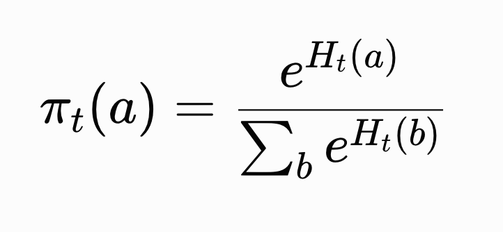
So far we’ve estimated action values Q(a) and then chosen actions with ε-greedy or UCB. Gradient bandits take a different route: instead of estimating how good each action is, they learn a preference H(a) for each action and turn those preferences into a probability distribution with the softmax (image 1):

Preferences have no units of reward, only relative differences matter. That makes the method robust to reward scaling and shifting.

The preferences are updated by stochastic gradient ascent on expected reward. After taking action A_t and observing reward R_t, we move the selected preference up (or down) relative to a baseline R̅_t (the average reward seen so far) and move the other preferences in the opposite direction (image 2):

When the reward is above the baseline the selected action becomes more probable; when it is below, it becomes less probable. As preference differences grow, the policy naturally concentrates on the better actions while still leaving a little probability mass on the others: a built-in exploration → exploitation transition.

This is the multi-armed-bandit special case of the REINFORCE policy-gradient theorem with a baseline.

#rl365

[Ian Murray @ianmurray33]

Learning Reinforcement Learning (Day 11/365)

Upper Confidence Bound Action Selection

Today we explore a new way of introducing exploration into our action selection. Recall that our previously-discussed exploration technique was epsilon-greedy action selection, where, with some probability epsilon, we decide not to take the greedy action and instead choose an action at random. While this often performs better than pure greedy action selection as the agent can avoid getting stuck on a suboptimal arm because of early unlucky estimates, it is somewhat of a coarse method of exploration.

What if instead we chose to explore based on how good a non-greedy action could be? This idea is formalized in a concept called Upper Confidence Bounds.

The core idea behind UCB is to add an element of uncertainty to our estimates of any action’s value. When we decide to pick an action, we take into account this uncertainty and the action’s potential to be optimal. When we select an action, we become more certain of its true value as we collect more data. When we don’t select an action, this uncertainty term grows. This drives natural exploration and eventually helps us converge on better action value estimates as more actions are sampled and their values estimated, making ultimate greedy selections based on more robust estimates of which action is optimal versus not.

#rl365

[Ian Murray @ianmurray33]

Learning RL (Day 10/365)
Non-Stationary Rewards and Constant Step-Size α

So far we've only looked at stationary k-armed bandits: the reward distributions never change. That's great for understanding the mechanisms of agents in these k-armed bandit settings, but real-world RL problems often involve non-stationarity.

When the rewards drift, sample-average estimation (α = 1/n) starts to fail. Once n is large, each new reward barely moves Q. Old data bury the new evidence.

A solution is to keep α constant: Q <-- Q + α(R-Q)
This is called recency-weight exponential average, as rewards are weighted with α(1-α)^k, causing distant rewards to fade exponentially (how quickly depends on α, shown in the video).
Larger α = shorter memory, reacts fast and noisier. Smaller α = longer memory, smoother, but lags

α = 1 uses only the latest reward. Clever selection of the α parameter value will depend on how quickly the rewards change in the particular environment.

#rl365

[Ian Murray @ianmurray33]

Hey Stash, would love to take a swing at the application - my dad and I do a lot of work in his yard and it would be so sick to have a robo dog to help us out!

Just getting my feet wet in RL and robotics, no better way to learn than through cool projects :)

https://t.co/FEsPpOSFof

[Ian Murray @ianmurray33]

@mrfundman Could you add me as well please! Thank you

[Bryan @BryanAguir33]

In Search Of clothes on https://t.co/qynJ6AO3OG

[Ian Murray @ianmurray33]

There's a cool company doing this in the OT space called Dispel (https://t.co/nUSymdg6tC) - their "moving target defense" solution spins up a bunch of VMs in commercial clouds/hyperscalers that serve as nodes to route remote-access traffic - makes it both hard to identify what network route the critical traffic is taking and exploit any holes in the network while it is transmitting before it gets recycled - network-focused and not source-code specific like u mention but really cool stuff esp for the ancient protocols that OT environments rely on - not sponsored :)

[Ian Murray @ianmurray33]

@Keanaalabre Interested! Just sent a DM

[Ian Murray @ianmurray33]

@johnbai Hope to see everyone there 🤞

[Ian Murray @ianmurray33]

Learning Reinforcement Learning (Day 9/365)

Incremental Implementation

I spent time re-reading the Sutton and Barto chapter and missed incremental implementation, which is an important subject for future lessons like upper confidence bounds (UCB) and dealing with non-stationary reward distributions.

As a recall, the sample average value estimation equation simple takes an average of all past rewards to estimate the value for a particular action.

Q_n+1 (a) = (R_1 + R_2 + R_3 + ... + R_n) / n

While this is perfectly adequate for calculating this estimate, there are some drawbacks that can be improved upon. When considering how we would implement this for computation, you will discover that updating our value estimation for Q(a) will require:
A. Memory that scales with the number of rewards
B. Computation time that similarly scales with the number of rewards

Memory scales linearly because we need to store all past rewards (R_1, R_2, ... , R_n) which correlates with n.

Computation scales linearly because we take a sum of all rewards, adding each reward to the running sum until we have summed all n rewards, then take a computation step to calculate the quotient (R_1 + ... + R_n) / n

We can improve this with incremental implementation, which is an update rule that is derived from our standard sample average formula (see video).

The final update rule is:
Q_n = Q_{n-1} + (1/n)*[R_n - Q_{n-1}]

This may look familiar to folks who have done stats or ML. The "psuedocode" version of this is:

NewEstimate <-- Old Estimate + StepSize * [Target - OldEstimate]

The expression [Target - OldEstimate] is known as the error, and the StepSize parameter is commonly denoted as alpha (α). In the case of our sample average value estimate, alpha is (1/n). This value becomes smaller as n grows, which means that as we receive more rewards and continue taking actions (i.e. increase n), the updates that are made to our value estimate become smaller and smaller, which is helpful towards converging on an estimate. Keeping the step size as (1/n) is exactly *why* value estimation is an average - it equally weights all rewards. In the next lesson we will show what happens when we apply a constant step size parameter, creating recency-weighted averages which is critical for properly estimation reward distributions that change over time.

#rl365

[Ian Murray @ianmurray33]

Hey Rob - would love to connect. Sparknotes on me:
- ex-Tesla data science, prior experience full stack eng at startups
- spent last 2 years sourcing and interfacing with ceos/founders at a growth equity firm, and have spent free time building internal agent tools (slackbots and in our proprietary CRM). Coverage area is AI/ML + infra
- Looking to get back into tech world - strength of mine is leveraging tech & client facing skills to both build product and communicate business value with non-tech stakeholders

NYC-based - would love to explore if there might be a fit

[Ian Murray @ianmurray33]

Learning Reinforcement Learning (Day 8/365)

Preface: Given some wonderful audience feedback, I will start to include a sentence or two per post hitting on the core intuition for the discussed concept, such that folks can grasp the idea if the jargon/notation is unfamiliar.

Yesterday I showed how the greedy approach fails: start both estimates at zero, pull one lever, get a positive reward, and now that lever is the only one that ever looks good again. The other arm sits at zero forever, untouched.

I flagged in that post that setting the initial estimates to 0 is what drives the behavior. As soon as a reward is sampled, and we update our estimations, any positive reward will always be picked against an un-tested distribution that we estimate to provide zero reward. This creates the loop that we never escape from.

This can be alleviated with a concept called optimistic initial values (OIV). The core intuition behind OIV is essentially: "why don't we set our initial estimation to a ridiculously high value? Every lever arm/distribution looks amazing before we touch it. Our greedy selection, which picks the lever we think gives the highest reward, will cause to pull each arm at least once." From there, the agent follows the greedy selection over honest estimates.

This is exploration falling out of the simple fact that our estimates are too high to start. It's an instance of a broader principle seen frequently in RL: optimism in the face of uncertainty - when you don't know how good something is, assume it's great and make reality talk you down.

A few bullets to caveat this technique of optimistic initial values:
1. Setting the optimistic values requires some knowledge of the reward scales, and thus some prior knowledge about the problem you are solving
2. It's one-time: the optimism is "spent" in the first few pulls, and does not return again once we have more accurate estimates of the rewards
3. If the distribution that yields your rewards is non-stationary (i.e. changes over time), then you will need exploration that recurs, which OIV doesn't provide

Next time we will get into a "smarter" form of optimism: upper confidence bounds (UCB)
--
#rl365

[Ian Murray @ianmurray33]

@mert_gulsun @FrancescoSacco1 if you are looking to learn more about k-armed bandits, please consider checking out this thread- has some nice animations to help with intuition (i'm a visual learner :) )

https://t.co/pZQgbHI15f

&lt;end self-plug&gt;

[Ian Murray @ianmurray33]

Learning Reinforcement Learning (Day 7/365)
(Thread post today)

This one will extend the discussion on bandit algorithms and epsilon-greedy methods, with some visualizations that hopefully drive the intuition home.

As a refresher of the k-armed bandit problem: a "bandit" is a slot machine. A k-armed bandit is k of them, or one machine with k levers. Each lever pays out a reward drawn from its own fixed distribution, and those distributions are hidden from you. You don't know which lever is best; the only way to learn anything is to pull one and see what you get.

You get a limited number of pulls. The whole problem is this: how do you spend them to walk away with the most total reward?
--
This first animation shows how sampling helps develop an estimation of this stationary distribution of rewards. With infinite samples, we could reach q*(a) = Q(a), i.e. our estimation of the population reward being the mean of population reward itself, but this is obviously impractical.

So instead, we average our samples over however many we've taken to reach our best guess. With a single-armed bandit, there is no idea of choice, we simply sample from the same distribution and approximate what the reward is. 🧵

[Ian Murray @ianmurray33]

This segues us nicely to a simple solution to this issue - the "epsilon-greedy" approach. The core of this approach is: most of the time, select the greedy action (i.e. pull the lever with the highest estimated reward given what we know). Then, on some occasions, sample uniformly across all possible levers/distributions, and sample from the randomly selected one.

The rate at which we choose this uniformly-random lever is dictated by our choice of epsilon - so if we set epsilon to be 0.1 or 10%, then roughly 1 in 10 samples we will explore.

The video helps visualize how this simple technique can cause use to avoid the pitfall of blind exploitation, and over enough samples, help us build more robust estimations of each. There is a fair amount of nuance in the choice of epsilon and the implications that result, as well as other ideas related to bandit algorithms (optimistic initial values, and upper confidence bounds) that we will explore in the coming days.

If you found the videos helpful, please let me know - they are built using @3blue1brown's wonderful manim library and are relatively easy to cook up with the help of Cursor.

[Ian Murray @ianmurray33]

Learning Reinforcement Learning (Day 7/365)
(Thread post today)

This one will extend the discussion on bandit algorithms and epsilon-greedy methods, with some visualizations that hopefully drive the intuition home.

As a refresher of the k-armed bandit problem: a "bandit" is a slot machine. A k-armed bandit is k of them, or one machine with k levers. Each lever pays out a reward drawn from its own fixed distribution, and those distributions are hidden from you. You don't know which lever is best; the only way to learn anything is to pull one and see what you get.

You get a limited number of pulls. The whole problem is this: how do you spend them to walk away with the most total reward?
--
This first animation shows how sampling helps develop an estimation of this stationary distribution of rewards. With infinite samples, we could reach q*(a) = Q(a), i.e. our estimation of the population reward being the mean of population reward itself, but this is obviously impractical.

So instead, we average our samples over however many we've taken to reach our best guess. With a single-armed bandit, there is no idea of choice, we simply sample from the same distribution and approximate what the reward is. 🧵

[Ian Murray @ianmurray33]

There's a seemingly obvious answer, explored in this post: pull the lever that you think gives you the highest reward! This is called the "greedy" approach, where you constantly exploit what you know.

This comes with pitfalls, outlined in this post's video - namely, when starting with two distributions of unknown reward, you might set the initial estimates to zero. Then, pulling from one of these distributions immediately updates your estimate to be non-zero. From that point on, following the greedy algorithm naively, you will sample only from that distribution, as whatever that Q(x) is will necessarily be higher than your Q(y) estimate of 0.

(Setting the starting estimations at 0 does drive this behavior, and can be mitigated with a technique called "optimistic initial values", which we explore later)