mr_atari

Ich schreibe über Freiheit, Philosophie und Ökonomie.
Ab und zu mal etwas zum Klimascam.

[mr_atari @mr_atari77]

10 Gebote eines Liberalen

1. Lebe frei und lasse andere frei leben.
2. Du sollst keine Gewalt gegenüber anderen Menschen üben, es sei denn, es ist zur Verteidigung von Leben, Freiheit oder Eigentum notwendig.
3. Du sollst nicht töten.
4. Du sollst nicht stehlen.
5. Du sollst kein falsches Zeugnis reden wider deinen Nächsten.
6. Du sollst nicht begehren Deines Nächsten Partner, Haus, Auto oder sonst irgendetwas aus seinem Besitz.
7. Du sollst Deine Eltern und Vorfahren ehren.
8. Du sollst andere Menschen behandeln nach ihrem Verhalten und nicht nach ihrer Abstammung, Identität oder Religion.
9. Du sollst nicht nur an Dich selbst denken, sondern auch an Deine Mitmenschen.
10. Du sollst Deine Vertretung weise wählen und stets kontrollieren, dass sie nicht zu viel Macht erlangen.

Diese Gebote sollen liberale UND christliche Werte wie Freiheit, Gewaltlosigkeit, Solidarität, Verantwortung, Nächstenliebe, Gerechtigkeit und Integrität unterstützen.

Und Damit diese Gebote auch weitergetragen werden, macht ein zusätzliches Gebot Sinn:

11. Du sollst diese Gebote ehren und an Deine Nachkommen weitergeben.

[Max Stirner @ernsterjuenger]

😁

[mr_atari @mr_atari77]

Interessant. Ich kannte die Geschichte.
Außer den Teil mit den drei Körben.

[Students For Liberty @sfliberty]

Three iron cages hang from a church tower in the German city of Münster. They have been there for almost 500 years.

Inside them, once, were the bodies of men who tried to build heaven on earth by abolishing private property.

Münster wants its people to know what put them there. 🧵

[Andrei Illarionov @AnIllarionov]

The American economic miracle

Andrei Illarionov
July 3, 2026

The American economic miracle stands out as one of the most remarkable accomplishments in the United States’ 250-year history.

The idea of an “Economic Miracle” and the criteria used to define it.
The term “economic miracle”—which entered global academic and public discourse after World War II—traditionally refers to a country’s economic success in achieving and sustaining high rates of economic growth over a significant period.

The most well-known examples of economic miracles are the cases demonstrated in the post-war decades by Germany, Italy, Japan, South Korea, Taiwan, Hong Kong, Singapore, China, and Ireland.

The primary criteria for identifying an economic miracle are:
- high rates of national economic growth (exceeding the global average);
- the sustainability of these high growth rates—that is, maintaining them for a specific period, lasting at least one decade.
Achieving and sustaining economic growth rates above the global average naturally increases the national economy’s share of the global economy. Thus, a change (specifically, an increase) in the national economy’s share of global GDP can also serve as an aggregate indicator of an economic miracle.

The American Economic Miracle: Quantitative Parameters
The first criterion of an economic miracle is an economic growth rate that exceeds the global average.

Over the 250-year period from 1775 to 2025, U.S. GDP increased 3,515-fold. No other state in existence at the end of the 18th century—nor any other state with a population exceeding 30 million in 2025—has achieved such a result.

The growth index of the American economy over this 250-year period exceeded the growth index of the entire global economy by a factor of 20.7.

GDP growth indices in selected countries worldwide, 1775–2025
Country Growth, times Exceeding the global economic growth index, times
United States 3515 20.72
Finland 365 2.15
Mexico 335 1.98
Peru 288 1.70
South Africa 268 1.58
Sweden 165 0.97
Germany 104 0.61
United Kingdom 100 0.59
Italy 95 0.56
France 61 0.36
World total 170 1.00
Sources: Maddison Project Database, 2023, Colonial Dates Dataset, 2019, IMF Database, World Bank Database

A second criterion for an economic miracle is maintaining economic growth rates above the global average over an extended period. The European and East Asian economic “tigers” sustained above-average growth rates for two, three, or four decades—and China for nearly five.

In contrast, the United States demonstrated above-average economic growth rates for an unprecedented duration: 155 years, from 1790 to 1945.

A comprehensive criterion for an economic miracle is an increase in the national economy’s share of global GDP. Between 1775 and 1945, the U.S. share of the global economy rose from 0.71% to 30.94%—an extraordinary increase of 30.2 percentage points of global GDP. No other country in the world has managed to increase its share of the global economy to such an extent over a similar period.

Components of U.S. Economic Success
In strictly mathematical terms, the volume of GDP produced is multiplication of the employed population by that population’s labor productivity. Another way to express GDP volume is multiplication of the total population (which correlates closely with the employed population) by GDP per capita (which correlates closely with GDP produced per employed person—i.e., labor productivity). In other words, the two most important factors determining the volume of GDP produced are population size and GDP per capita.

Over the course of 250 years, the U.S. population grew 138-fold. By this metric, the United States ranks near the top globally, although several dozen countries do surpass it in this regard. Nevertheless, the country’s significant population growth—particularly during its first 175 years (between 1775 and 1950) — contributed substantially to its rapid economic expansion and to the rising share of the U.S. in both the global population and the global economy.

It should also be noted that, since 1950, the U.S. share of the global population has steadily declined. Consequently, the net contribution of the demographic factor to changes in the U.S. share of the global economy has been negative over the past 75 years.

A far more significant contribution to the “American miracle” phenomenon came from steadily rising GDP per capita relative to the global average. Between 1775 and 1999, U.S. GDP per capita increased 18.4-fold (compared with a 9.5-fold increase globally). It was precisely this growth in per capita GDP—outpacing global averages and serving as a proxy for labor productivity—between 1790 and 1945 that played the decisive role in creating and sustaining the “American miracle” for 155 years.

The American economic miracle, the American global leadership, and the American economic golden age
By applying the previously defined criterion for an economic miracle—a more or less steady growth in the nation’s share of global GDP over a long period—we can pinpoint the timeframe that fits this condition: that is, the 155-year span from 1790 to 1945.

During the lifetime of this economic miracle, the rapidly growing U.S. economy surpassed the size of the following economies:
- the Russian Empire in 1854,
- the United Kingdom in 1862,
- India in 1868, and
- China in 1882.

From 1882 onwards, the U.S. economy became the undisputed global leader in terms of GDP size.

The United States maintained this leadership until 2013. In 2014 China’s GDP (adjusted for purchasing power parity) surpassed that of the US for the first time. Thus, the period of American global economic leadership (in terms of absolute GDP) spanned 132 years, from 1882 to 2013.

Regarding the key driver of economic growth—GDP per capita—the U.S. definitively overtook the UK in 1899, following roughly two decades of figures that closely mirrored Britain’s.

Over the ensuing century—up to 1999—and despite various fluctuations (driven by both economic conditions and geopolitical upheavals), the U.S. managed not only to maintain a GDP per capita above the global average but even to widen the gap between itself and that average.

It is precisely this period—from 1899 to 1999—that can be termed the American “economic golden age.”

It should be noted that between 2000 and 2025, all indicators of U.S. economic dynamics (GDP growth rates, GDP per capita growth rates, population growth rates, and the national economy’s share of global GDP) have declined significantly and consistently, falling below global averages. The reasons for U.S. economic success during its first centuries of existence, as well as the causes of the significant slowdown in the American economy over the last quarter-century, warrant a separate analysis.

Conclusion
One can outline the chronology of key periods in 250-year U.S. economic history:
- 1790–1945 (155 years) – the American economic miracle;
- 1882–2013 (132 years) – American global economic leadership (by absolute GDP volume);
- 1899–1999 (101 years) – the American “economic golden age,” marked by US global leadership in terms of both GDP per capita and the steadily widening gap between this American figure and the global average.
https://t.co/fzK7yMeZHc
https://t.co/XaZ3TCBpdA

[mr_atari @mr_atari77]

@sfliberty It's not even capable of redistributing wealth.
Wealth sticks at the greedy fingers of politicians and wealthy people, which find an arrangement with politics on the expense of ordinary people.

It's basically a satanic cult.

[mr_atari @mr_atari77]

@kreitz_steffen Ich denke nicht, dass man mehrere 100k nach dem Prinzip Hoffnung bezahlt.
Da sind handfeste Deals eingeplant.

[mr_atari @mr_atari77]

Homer Simpson, bist du das?

[Brian Roemmele @BrianRoemmele]

90% Of His Brain Was Missing And No One Knew It.

—

In 2007 in France, a 44-year-old man went to the doctor complaining of numbness in his leg and underwent a brain CT scan that revealed a shocking truth.

That man didn't have 90% of his brain. The skull was almost entirely filled with cerebrospinal fluid and all that remained of the brain was a thin peripheral portion surrounding the skull.

Yet that man, whose IQ was just below average (IQ 75), had been leading a normal life for years: he was married, had two children, a job and was obviously aware of himself, he moved, laughed, loved and ultimately he lived.

The case shocked the world scientific community and was described in the prestigious Lancet journal, becoming the subject of questions and amazement.

The evidence of the facts raised, as can easily be imagined, many questions about the very concept of consciousness, understood as "awareness of the self" and the possibility of leading a normal life practically without a brain.
The patient's clinical history was reconstructed and it was discovered that he was born suffering from a form of hydrocephalus.

For this reason, a few months before his life, a cerebral shunt was inserted into his skull, capable of draining excess cerebrospinal fluid. That shunt was removed at the age of 14 and the patient, after an initial series of problems that had caused paresis in his left leg, was eventually able to resume an almost normal life and had completely forgotten about the problem.

Over the next 30 years, the liquor began to invade the skull again and progressively erode the brain (90% of the brain!), leading to that feeling of weakness in the leg which prompted the patient to undergo a medical examination. at the age of 44.

But all this was not able to explain how the brain invaded by cerebrospinal fluid and eroded by 90% of its volume had "known" to recalibrate itself over the years, allowing him to lead a normal life anyway.

Axel Cleeremans, a cognitive psychologist at the Université Libre of Brussels, Belgium, attempted to answer these questions in 2016 during a conference of the Association for Scientific Studies on Consciousness, held in Buenos Aires.

According to Cleeremans, the case of the French patient had demonstrated the extraordinary "readaptation capacity" of the human brain. The frontal, parietal, temporal and occipital lobes of the brain, in fact, preside over the main cognitive and perceptive functions, yet in the patient they were practically completely absent and this demonstrated that the brain of that man - and therefore of every man - had been able to "move" those functions to the residual perimeter section of 10%.

The second ability that was made evident by the clinical case under examination was the "plasticity of the brain". According to Cleeremans' hypothesis, "self-awareness" (or detailed self-cognition) is formed through experience, the relationship between oneself and the surrounding world and learning, and is subject to continuous modifications and adjustments in course of life.

The case of the French man who lived a normal life until the age of 44 without 90% of his brain demonstrated to science a fact that had until then been unknown, namely that just 10% of the brain tissue is sufficient to re-elaborate a “theory of the self” and to make that person a man in all respects.

We can’t even begin to know what we don’t know…

For the Reddit “actually” debunker types. Read this before you move your thumbs: https://t.co/m2qsol172F

[mr_atari @mr_atari77]

Abstimmungen

Demokratie wird im Alltag oft auf einen simplen Mechanismus reduziert: Abstimmungen durch Wahlen. Mehrheit gewinnt, Minderheit verliert. Dieses Bild ist eingängig – und zugleich verkürzt. Eine politische Ordnung, die sich ausschließlich an Mehrheitsentscheidungen orientiert, trägt ein strukturelles Risiko der Degradation in sich.

Abstimmungen sind ein Werkzeug. Vor allem ein Werkzeug zur friedlichen Beilegung von Konflikten. Sie sind nicht das Prinzip.

Der Einwand liegt nahe, dass Demokratie gerade in der Gleichheit der Stimmen ihren moralischen Kern habe. Doch Gleichheit der Stimmrechte ist eine Verfahrensregel, keine inhaltliche Garantie von Gerechtigkeit.

Die amerikanischen Gründerväter hatten ein tiefes Misstrauen gegenüber der Vorstellung, dass Mehrheiten automatisch gerecht entscheiden.

Dass die Wünsche der Mehrheit des Volkes oft auf Ungerechtigkeit und Unmenschlichkeit gegenüber der Minderheit gerichtet sind, wird durch jede Seite der Weltgeschichte belegt.
John Adams

und:

In dem Moment, in dem in einer Gesellschaft die Vorstellung akzeptiert wird, dass Eigentum nicht ebenso unantastbar ist wie die Gesetze Gottes [...], beginnen Anarchie und Tyrannei.
John Adams

und weiter:

Wenn „Du sollst nicht begehren“ und „Du sollst nicht stehlen“ keine Gebote des Himmels wären, dann müssten sie zu unverletzlichen Grundsätzen in jeder Gesellschaft gemacht werden, bevor diese zivilisiert oder frei sein kann.

Mehrheit bedeutet Macht – aber nicht moralische Legitimation.
Eine Abstimmung kann entscheiden, WER regiert.
Sie darf nicht entscheiden, WAS grundsätzlich rechtmäßig ist.
Wenn keine moralischen und institutionellen Schranken gesetzt werden, wird Demokratie zur organisierten Plünderung.

Das betrifft nicht nur Abstimmungen über Eigentumsfragen. Libertäre und klassisch-liberale Denkschulen weisen seit Langem darauf hin, dass nach dem Prinzip “Ein Mensch, eine Stimme" Personen über Dinge abstimmen, für die sie keine Verantwortung tragen.

Ein besonders krasses Beispiel liefert der russische Angriffskrieg auf die Ukraine. Eines der größten Hindernisse für einen Waffenstillstand sind russische Forderungen nach Gebietsabtretungen. Die Ukrainische Verfassung sieht für so einen Fall ein obligatorisches Referendum vor. Damit dürfen, zumindest theoretisch, Menschen, die selbst nie an die Front kommen werden, über Leben und Tod der Soldaten in den Schützengräben entscheiden. Jedenfalls, wenn es jemals zu einem Referendum zu diesem Thema in der Ukraine kommen sollte.

Das ist zutiefst unmoralisch.

Eine ungefilterte Demokratie ist damit keine ideale Staatsform, sondern eine instabile:

Eine einfache Demokratie. . . ist eines der größten aller Übel.
Benjamin Rush

Was hier wie eine Provokation klingt, ist in Wahrheit eine nüchterne Analyse.
Eine reine Abstimmungsdemokratie kennt keine strukturellen Schranken:

Emotion schlägt Vernunft
kurzfristige Interessen schlagen langfristige Stabilität
Mehrheiten entdecken ihre Fähigkeit, sich selbst zu begünstigen

Die zentrale Einsicht der Gründerväter war dabei von ernüchternder Klarheit:
Nicht nur Könige neigen zum Machtmissbrauch – auch das Volk. Das ist eine der Begründungen, warum unser Grundgesetz so wenig direktdemokratische Elemente enthält. Repräsentation wurde gestärkt, um Entscheidungen zu verlangsamen, zu filtern und in institutionelle Verantwortung einzubetten.

Doch genau hier entsteht ein zweites Problem, das oft unterschätzt wird.

Repräsentation bedeutet immer auch Informationsasymmetrie, eine strukturelle Distanz zwischen Entscheidung und Verantwortung, sowie Eigeninteressen der Entscheidungsträger. Die Gefahr verschiebt sich lediglich. Von der Tyrannei der Mehrheit - zur möglichen Verselbstständigung der Repräsentanten. Damit entsteht ein Spannungsfeld, das sich nicht auflösen lässt. Wir haben es wieder mit einer klassischen Trade-Off Situation zu tun.

Die Gründerväter der USA verstanden Demokratie nicht als Herrschaft der Mehrheit allein,
sondern als ein System zur Kontrolle von Macht.

Abstimmungen sind darin ein notwendiges Element.
Aber sie sind niemals das Fundament.

[mr_atari @mr_atari77]

@kallweit_heiko Jordan Peterson, Biblical Series

https://t.co/2DJcK6cvUV

[mr_atari @mr_atari77]

@Joe_0_ @tobibog Wenn ein besserer Fernseher zum gleichen Preis verkauft wird, dann ist das aufgrund gestiegener Produktivität. D.h. irgendwo anders wurde Arbeitskraft frei um mehr Güter herzustellen.
Qualitatives Wachstum ganz ohne Statistik Voodoo.

[mr_atari @mr_atari77]

@libertaeredeju Sozialismus: Eine Idee, so überragend, dass sie mit Gewalt eingeführt werden muss.

[mr_atari @mr_atari77]

@Joe_0_ @SHomburg Ja, das kann wachsen durch Software und Dienstleistungen. Braucht keine Rohstoffe.

[mr_atari @mr_atari77]

Das Wachstum kann auch rein qualitativ sein, ohne dass es großartig mehr Ressourcen braucht.

Und selbst quantitatives Wachstum ist noch ohne Ende möglich. Die chemischen Elemente werden durch menschliche Nutzung janicht "verbraucht", nur umgewandelt.
Der Planet ist viel größer als die meisten sich vorstellen. Die Natur auch.
Und wenn das nicht reicht, gibt es noch das Sonnensystem. Alles nutzbar, ohne die Schöpfung kaputtzumachen.

[mr_atari @mr_atari77]

@ziv_ravid Tried this a year ago. Has not worked yet. Was wildly hallucinating.

Have you used a specialized model?

[mr_atari @mr_atari77]

"It's a curve fitting exercise, rather than physics".

[Chris Martz @ChrisMartzWX]

Have you seen the figure on the left before?

Chances are you have if you’re actively involved in the climate change debate. If not, let me break it down.

The figure, adapted from Figure SPM.1 in the IPCC AR6 Summary for Policymakers, is often touted as the “smoking gun” that proves virtually all observed global warming since 1850 is due to mankind’s greenhouse gas (GHG) emissions. The figure implies that global climate models (GCMs) skillfully reproduce observed warming (see black curve) since the “pre-industrial” era. They claim that this chart is synthesized from “multiple lines of evidence,” and that GCMs cannot skillfully reproduce the observed temperature trends without extra GHGs.

🔗https://t.co/5lspFokYOu(p. 6)

However, this graph is not the “smoking gun” that many people think it is. So, let me explain why.

First, it’s important to understand exactly what Figure SPM.1 is showing.

⬛️ 𝗖𝘂𝗿𝘃𝗲: The observed global mean surface [air] temperature (GMST) anomaly (1850–2019) from four surface station-based datasets. It shows ~1.2°C of warming since 1850, though there is slight divergence between datasets (e.g., Berkley Earth, HadCRUT, NOAA, etc.). The likely range falls between 1.1–1.3°C, and I do not dispute these estimates, although I do not care much about what the GMST is.

🟩 𝗖𝘂𝗿𝘃𝗲: The CMIP6 multi-model mean (MMM) GMST response to natural forcings and internal variability only. These are primarily solar forcing (e.g., changes in total solar irradiance, which is a measure of the solar power over all wavelengths per unit area incident at the top of the atmosphere), stratospheric aerosol injection (SAI) from major volcanic eruptions (think Mount Tambora, 1815; Krakatoa, 1883; El Chichón, 1982; or Mount Pinatubo, 1991), and the El Niño Southern Oscillation (ENSO).

🟦 𝗖𝘂𝗿𝘃𝗲: Simulated GMST response due to aerosol forcing only. Aerosols are fine solid or liquid particles—natural or anthropogenic in origin—that are suspended in the air and generally have diameters of <1 μm (1 × 10⁻⁴ cm). Depending on type, aerosols can either act to warm or cool the Earth’s atmosphere. For instance, bright aerosols (e.g., sulfate particulates from coal burning) scatter incoming solar radiation back to space, which causes net cooling. Dark aerosols (e.g., black carbon from diesel exhaust), on the contrary, absorb incoming sunlight, resulting in net warming.

🟥 𝗖𝘂𝗿𝘃𝗲: Simulated ensemble GMST response to manmade GHG emissions only. These primarily are carbon dioxide (CO₂) and methane (CH₄), and to a lesser extent, include ozone (O₃) and nitrous oxides (NOx).

⬜️ 𝗖𝘂𝗿𝘃𝗲: Simulated GMST change due to natural forcings / variability + aerosols + GHGs. In other words, it’s the sum of the green, blue, and red curves.

As we can see below, the IPCC’s figure implies that GCMs have done remarkably well to explain why the globe has warmed [𝘴𝘭𝘪𝘨𝘩𝘵𝘭𝘺] since 1850. The verdict, so we’re told, is that GHG emissions from our energy consumption, industrial activities, and transportation are squarely to blame. And who’s going to argue with that? After all, scientists and climate activists routinely tell us that “It’s just basic physics” and that “The science is settled.”

There’s just one problem: the conclusion depends heavily on GCMs whose historical behavior (called hindcasting) is not an independent test in the way that the general public has been misled to believe by much of the scientific community.

GCMs are not simply pure radiative physics machines that can be turned on, run out to a certain date, and allowed to speak for themselves. They contain many parameterized processes such as cloud feedbacks, aerosol forcing, convection, land-surface exchanges, and ocean-atmosphere coupling that must be calibrated during model development.

1️⃣ 𝗖𝗟𝗜𝗠𝗔𝗧𝗘 𝗠𝗢𝗗𝗘𝗟𝗦 𝗦𝗧𝗥𝗨𝗚𝗚𝗟𝗘 𝗪𝗜𝗧𝗛 𝗡𝗔𝗧𝗨𝗥𝗔𝗟 𝗩𝗔𝗥𝗜𝗔𝗕𝗜𝗟𝗜𝗧𝗬

Paleoclimate proxies (e.g., tree rings, ice cores, and sediments) show significant multidecadal to centennial temperature fluctuations in pre-industrial times. The Greenland and Antarctic ice core-based temperature reconstructions, for instance, make that abundantly clear.

🔗https://t.co/5PpWXs3cak

The models in CMIP5/6 smooth temperature curves and fail to reproduce the known amplitude of natural internal variability exhibited in multiple temperature reconstructions both regionally and globally (i.e., the more accurate pre-Hockey stick reconstructions). So, when modelers claim that natural forcing and internal variability cannot explain any warming since 1850, we should ask: Is that because nature truly could not have contributed much? Or is it possible that GCMs underrepresent natural variability?

That's not a trivial distinction.

2⃣ 𝗖𝗟𝗜𝗠𝗔𝗧𝗘 𝗠𝗢𝗗𝗘𝗟𝗦 𝗔𝗥𝗘 𝗔𝗥𝗧𝗜𝗙𝗜𝗖𝗜𝗔𝗟𝗟𝗬 𝗧𝗨𝗡𝗘𝗗

Because GCMs struggle to independently reproduce observed historical temperature variations, modelers often pre-tune parameters (turn “knobs”) until the GMST output aligns with the observed GMST record.

This is not a conspiracy theory; it’s a demonstrable fact. The question is not whether tuning occurs. It does. The question is how much confidence we should place in attribution claims when models are essentially fudged to agree with the same historical record that is later used to demonstrate their alleged success.

Figure 3.8 on the right from IPCC AR6 WG1 illustrates this perfectly. It shows the assessed contributions to global warming from GHGs, aerosols, and natural forcings / internal variability over the period 2010–19 minus 1850–1900.

Let’s break it down:

🟩 The green boxes in Figure 3.8 show the spread in modeled GMST change ascribed to natural forcing / internal variability. The MMM is centered around the zero mark with little variation between the individual models in the ensemble. This is, once again, due to the fact that GCMs cannot hindcast well. So, the modelers assume that natural contributions to warming must be near zero.

🟦 Aerosol effective radiative forcing (ERF) carries enormous uncertainty: the MMM suggests a modest net cooling of ~0.5°C, but the range spans from a strong cooling of –0.9°C to a weak warming of +0.1°C over the period 1850–2019. The uncertainty arises because it is unknown whether the net warming from black carbon is offset by the cooling from sulfate aerosols (H₂SO₄). The MMM of 0.5°C thus has a 100% margin of error, which means that no scientists know exactly how much aerosol forcing has dampened (or enhanced) GMST change.

Does that sound like “settled science” to you? It sure doesn’t to me.

But modelers need to reproduce warming of ~0.9°C to 1.1°C. If aerosol emissions result in net cooling, then that cannot be the cause. So, what do these modelers td? They jack up the GHG forcing.

🟫 Extra GHGs also have uncertainty, though the margin of error is smaller in these estimates. The MMM suggests a strong warming of 1.5°C ± ~45%. All this tells us is that “the experts” have no clue just how sensitive the climate system is to extra GHGs in the Earth’s atmosphere.

Add these forcings together and the ensemble mean output lands near observations.

🔗https://t.co/6RS5rVXTRZ (p. 440)

There’s just one problem. Different models can get similar historical warming curves that resemble observations, but they use different combinations of aerosol cooling and GHG warming. That means the match to observed temperature trends does not uniquely prove the exact partitioning between GHGs, aerosols, and natural variability. For example, a model with strong aerosol cooling requires strong GHG warming to offset it. A different model with weak aerosol cooling requires a weaker GHG warming. Both will produce near-identical GMST curves that have high correlation to observations, but one cannot put much stock into these coefficients. This is a curve fitting exercise rather than real physics.

Mauritsen & Roeckner (2020), for example, openly describe tuning the Max Planck Institute model (MPI-ESM1.2) to match historical warming by adjusting cloud feedbacks and targeting an equilibrium climate sensitivity (ECS) of ~3°C (this is the IPCC's “best estimate”). With the known physics of radiative heat transfer, MPI-ESM1.2 produced an ECS of 7°C, more than double their target. Therefore, the modelers arbitrarily adjusted the cloud parameter scheme until the model output aligned with GMST observations.

In the closing remarks of the paper, the authors of Mauritsen & Roeckner (2020) say,

🗨️ “𝘞𝘦 𝘩𝘢𝘷𝘦 𝘥𝘰𝘤𝘶𝘮𝘦𝘯𝘵𝘦𝘥 𝘩𝘰𝘸 𝙬𝙚 𝙩𝙪𝙣𝙚𝙙 𝙩𝙝𝙚 𝙈𝙋𝙄-𝙀𝙎𝙈𝟭.𝟮 𝙜𝙡𝙤𝙗𝙖𝙡 𝙘𝙡𝙞𝙢𝙖𝙩𝙚 𝙢𝙤𝙙𝙚𝙡 𝙩𝙤 𝙢𝙖𝙩𝙘𝙝 𝙩𝙝𝙚 𝙞𝙣𝙨𝙩𝙧𝙪𝙢𝙚𝙣𝙩𝙖𝙡 𝙧𝙚𝙘𝙤𝙧𝙙 𝘸𝘢𝘳𝘮𝘪𝘯𝘨; 𝘢𝘯 𝘦𝘯𝘥𝘦𝘢𝘷𝘰𝘳 𝙬𝙝𝙞𝙘𝙝 𝙝𝙖𝙨 𝙘𝙡𝙚𝙖𝙧𝙡𝙮 𝙗𝙚𝙚𝙣 𝙨𝙪𝙘𝙘𝙚𝙨𝙨𝙛𝙪𝙡. 𝘋𝘶𝘦 𝘵𝘰 𝘵𝘩𝘦 𝘩𝘪𝘴𝘵𝘰𝘳𝘪𝘤𝘢𝘭 𝘰𝘳𝘥𝘦𝘳 𝘰𝘧 𝘦𝘷𝘦𝘯𝘵𝘴, 𝙩𝙝𝙚 𝙘𝙝𝙤𝙞𝙘𝙚 𝙬𝙖𝙨 𝙩𝙤 𝙙𝙤 𝙩𝙝𝙞𝙨 𝙥𝙧𝙖𝙘𝙩𝙞𝙘𝙖𝙡𝙡𝙮 𝙗𝙮 𝙩𝙖𝙧𝙜𝙚𝙩𝙞𝙣𝙜 𝙖𝙣 𝙀𝘾𝙎 𝙤𝙛 𝘢𝘣𝘰𝘶𝘵 𝟯 𝙆 𝙪𝙨𝙞𝙣𝙜 𝙘𝙡𝙤𝙪𝙙 𝙛𝙚𝙚𝙙𝙗𝙖𝙘𝙠𝙨, 𝙖𝙨 𝙤𝙥𝙥𝙤𝙨𝙚𝙙 𝙩𝙤 𝙩𝙪𝙣𝙞𝙣𝙜 𝙩𝙝𝙚 𝙖𝙚𝙧𝙤𝙨𝙤𝙡 𝙛𝙤𝙧𝙘𝙞𝙣𝙜.”

🔗https://t.co/uBatWfdyvQ

🔗https://t.co/8Ntgszrz3a(p. 44 for IPCC ECS “best estimate” of 3 K)

The “basic physics” did not yield correct values, so the scientists arbitrarily turn knobs on various parameters until they get their desired result.

This transparency is useful, but it also exposes the problem. If a model is tuned to the instrumental GMST record, then its ability to reproduce the 20th-century temperature record cannot be treated as independent proof that the model has correctly identified the cause(s) of that warming. This is a circularity problem. It does not mean that GHGs have had no effect. They definitely have, at least to some extent. But one cannot confidently claim that all of the warming since 1850 has been anthropogenic because “the models match observations.”

Scientists also haven’t always been transparent about this. For decades, modeling centers refused to inform the public exactly how GCMs are calibrated. The IPCC subtly admitted this in Chapter 9 of AR5 WG1, stating,

🗨️ “𝘞𝘪𝘵𝘩 𝘷𝘦𝘳𝘺 𝘧𝘦𝘸 𝘦𝘹𝘤𝘦𝘱𝘵𝘪𝘰𝘯𝘴 (𝘔𝘢𝘶𝘳𝘪𝘵𝘴𝘦𝘯 𝘦𝘵 𝘢𝘭., 2012; 𝘏𝘰𝘶𝘳𝘥𝘪𝘯 𝘦𝘵 𝘢𝘭., 2013) 𝙢𝙤𝙙𝙚𝙡𝙡𝙞𝙣𝙜 𝙘𝙚𝙣𝙩𝙧𝙚𝙨 𝙙𝙤 𝙣𝙤𝙩 𝙧𝙤𝙪𝙩𝙞𝙣𝙚𝙡𝙮 𝙙𝙚𝙨𝙘𝙧𝙞𝙗𝙚 𝙞𝙣 𝙙𝙚𝙩𝙖𝙞𝙡 𝙝𝙤𝙬 𝙩𝙝𝙚𝙮 𝙩𝙪𝙣𝙚 𝙩𝙝𝙚𝙞𝙧 𝙢𝙤𝙙𝙚𝙡𝙨.. 𝘛𝘩𝘦𝘳𝘦𝘧𝘰𝘳𝘦, 𝘵𝘩𝘦 𝘤𝘰𝘮𝘱𝘭𝘦𝘵𝘦 𝘭𝘪𝘴𝘵 𝘰𝘧 𝘰𝘣𝘴𝘦𝘳𝘷𝘢𝘵𝘪𝘰𝘯𝘢𝘭 𝘤𝘰𝘯𝘴𝘵𝘳𝘢𝘪𝘯𝘵𝘴 𝘵𝘰𝘸𝘢𝘳𝘥 𝘸𝘩𝘪𝘤𝘩 𝘢 𝘱𝘢𝘳𝘵𝘪𝘤𝘶𝘭𝘢𝘳 𝘮𝘰𝘥𝘦𝘭 𝘪𝘴 𝘵𝘶𝘯𝘦𝘥 𝘪𝘴 𝘨𝘦𝘯𝘦𝘳𝘢𝘭𝘭𝘺 𝘯𝘰𝘵 𝘢𝘷𝘢𝘪𝘭𝘢𝘣𝘭𝘦.”

🔗https://t.co/z2jHU1IbkD (pp. 749-50)

This initial lack of transparency became the focus of an editorial in Science Magazine in October 2016,

🗨️ “𝘐𝘯𝘥𝘦𝘦𝘥, 𝘸𝘩𝘦𝘵𝘩𝘦𝘳 𝘤𝘭𝘪𝘮𝘢𝘵𝘦 𝘴𝘤𝘪𝘦𝘯𝘵𝘪𝘴𝘵𝘴 𝘭𝘪𝘬𝘦 𝘵𝘰 𝘢𝘥𝘮𝘪𝘵 𝘪𝘵 𝘰𝘳 𝘯𝘰𝘵, 𝙣𝙚𝙖𝙧𝙡𝙮 𝙚𝙫𝙚𝙧𝙮 𝙢𝙤𝙙𝙚𝙡 𝙝𝙖𝙨 𝙗𝙚𝙚𝙣 𝙘𝙖𝙡𝙞𝙗𝙧𝙖𝙩𝙚𝙙 𝙥𝙧𝙚𝙘𝙞𝙨𝙚𝙡𝙮 𝙩𝙤 𝙩𝙝𝙚 𝟮𝟬𝙩𝙝 𝙘𝙚𝙣𝙩𝙪𝙧𝙮 𝙘𝙡𝙞𝙢𝙖𝙩𝙚 𝙧𝙚𝙘𝙤𝙧𝙙𝙨—𝙤𝙩𝙝𝙚𝙧𝙬𝙞𝙨𝙚 𝙞𝙩 𝙬𝙤𝙪𝙡𝙙 𝙝𝙖𝙫𝙚 𝙚𝙣𝙙𝙚𝙙 𝙪𝙥 𝙞𝙣 𝙩𝙝𝙚 𝙩𝙧𝙖𝙨𝙝. ‘𝘐𝘵'𝘴 𝘧𝘢𝘪𝘳 𝘵𝘰 𝘴𝘢𝘺 𝘢𝘭𝘭 𝘮𝘰𝘥𝘦𝘭𝘴 𝘩𝘢𝘷𝘦 𝘵𝘶𝘯𝘦𝘥 𝘪𝘵,’ 𝘴𝘢𝘺𝘴 𝘐𝘴𝘢𝘢𝘤 𝘏𝘦𝘭𝘥, 𝘢 𝘴𝘤𝘪𝘦𝘯𝘵𝘪𝘴𝘵 𝘢𝘵 𝘵𝘩𝘦 𝘎𝘦𝘰𝘱𝘩𝘺𝘴𝘪𝘤𝘢𝘭 𝘍𝘭𝘶𝘪𝘥 𝘋𝘺𝘯𝘢𝘮𝘪𝘤𝘴 𝘓𝘢𝘣𝘰𝘳𝘢𝘵𝘰𝘳𝘺, 𝘢𝘯𝘰𝘵𝘩𝘦𝘳 𝘱𝘳𝘰𝘮𝘪𝘯𝘦𝘯𝘵 𝘮𝘰𝘥𝘦𝘭𝘪𝘯𝘨 𝘤𝘦𝘯𝘵𝘦𝘳, 𝘪𝘯 𝘗𝘳𝘪𝘯𝘤𝘦𝘵𝘰𝘯, 𝘕𝘦𝘸 𝘑𝘦𝘳𝘴𝘦𝘺.”

The Science Magazine article continues, stating that climate scientists had been reluctant to come clean about tuning practices for years because they feared that skeptics would use their practices against them to downplay global warming,

🗨️ “𝙁𝙤𝙧 𝙮𝙚𝙖𝙧𝙨, 𝙘𝙡𝙞𝙢𝙖𝙩𝙚 𝙨𝙘𝙞𝙚𝙣𝙩𝙞𝙨𝙩𝙨 𝙝𝙖𝙙 𝙗𝙚𝙚𝙣 𝙢𝙪𝙢 𝘪𝘯 𝘱𝘶𝘣𝘭𝘪𝘤 𝙖𝙗𝙤𝙪𝙩 𝘵𝘩𝘦𝘪𝘳 ‘𝘴𝘦𝘤𝘳𝘦𝘵 𝘴𝘢𝘶𝘤𝘦’: 𝙒𝙝𝙖𝙩 𝙝𝙖𝙥𝙥𝙚𝙣𝙚𝙙 𝙞𝙣 𝙩𝙝𝙚 𝙢𝙤𝙙𝙚𝙡𝙨 𝘴𝘵𝘢𝘺𝘦𝘥 𝘪𝘯 𝘵𝘩𝘦 𝘮𝘰𝘥𝘦𝘭𝘴. 𝙏𝙝𝙚 𝙩𝙖𝙗𝙤𝙤 𝙧𝙚𝙛𝙡𝙚𝙘𝙩𝙚𝙙 𝙛𝙚𝙖𝙧𝙨 𝙩𝙝𝙖𝙩 𝙘𝙡𝙞𝙢𝙖𝙩𝙚 𝙘𝙤𝙣𝙩𝙧𝙖𝙧𝙞𝙖𝙣𝙨 𝙬𝙤𝙪𝙡𝙙 𝙪𝙨𝙚 𝙩𝙝𝙚 𝙥𝙧𝙖𝙘𝙩𝙞𝙘𝙚 𝙤𝙛 𝙩𝙪𝙣𝙞𝙣𝙜 𝙩𝙤 𝙨𝙚𝙚𝙙 𝙙𝙤𝙪𝙗𝙩 𝙖𝙗𝙤𝙪𝙩 𝙢𝙤𝙙𝙚𝙡𝙨—𝙖𝙣𝙙, 𝙗𝙮 𝙚𝙭𝙩𝙚𝙣𝙨𝙞𝙤𝙣, 𝙩𝙝𝙚 𝙧𝙚𝙖𝙡𝙞𝙩𝙮 𝙤𝙛 𝙝𝙪𝙢𝙖𝙣-𝙙𝙧𝙞𝙫𝙚𝙣 𝙬𝙖𝙧𝙢𝙞𝙣𝙜. ‘𝘛𝘩𝘦 𝘤𝘰𝘮𝘮𝘶𝘯𝘪𝘵𝘺 𝘣𝘦𝘤𝘢𝘮𝘦 𝘥𝘦𝘧𝘦𝘯𝘴𝘪𝘷𝘦,’ [Bjorn] 𝘚𝘵𝘦𝘷𝘦𝘯𝘴[a director of the Max Planck Institute for Meteorology] 𝘴𝘢𝘺𝘴. ‘𝘐𝘵 𝘸𝘢𝘴 𝘢𝘧𝘳𝘢𝘪𝘥 𝘰𝘧 𝘵𝘢𝘭𝘬𝘪𝘯𝘨 𝘢𝘣𝘰𝘶𝘵 𝘵𝘩𝘪𝘯𝘨𝘴 𝘵𝘩𝘢𝘵 𝘵𝘩𝘦𝘺 𝘵𝘩𝘰𝘶𝘨𝘩𝘵 𝘤𝘰𝘶𝘭𝘥 𝘣𝘦 𝘶𝘯𝘧𝘢𝘪𝘳𝘭𝘺 𝘶𝘴𝘦𝘥 𝘢𝘨𝘢𝘪𝘯𝘴𝘵 𝘵𝘩𝘦𝘮.’”

🔗https://t.co/PImzcNbUQu

A fair test of GCM skill uses temperature data that the models are not pre-tuned to match, such as satellite-based lower tropospheric temperatures (TLT). CMIP6 models, initialized in 1979, show roughly TWICE the warming rate observed in the University of Alabama in Huntsville (UAH v6.0) TLT dataset as shown in the bottom right time series (e.g., Christy & McNider, 2017; Christy et al., 2018) Recent events, such as the strong El Niño, reductions in low- and mid-altitude stratiform cloud cover, and perhaps the Hunga Tonga eruption have narrowed the gap temporarily, but the systematic warm bias persists in many model simulations.

🔗https://t.co/zueJLn9sY4

🔗https://t.co/vUJgmigsAe

3⃣ 𝗧𝗛𝗘𝗥𝗘 𝗜𝗦 𝗔𝗡𝗧𝗛𝗥𝗢𝗣𝗢𝗚𝗘𝗡𝗜𝗖 𝗖𝗢𝗡𝗧𝗥𝗜𝗕𝗨𝗧𝗜𝗢𝗡; 𝗧𝗛𝗘 𝗠𝗔𝗚𝗡𝗜𝗧𝗨𝗗𝗘 𝗜𝗦 𝗨𝗡𝗖𝗘𝗥𝗧𝗔𝗜𝗡

No serious analysis denies that there is some human influence on global warming. It is a scientific fact that CO₂ absorbs infrared radiation. Increasing CO₂ changes the radiative balance of Earth’s atmosphere. All else equal, that produces a warming tendency in the lower atmosphere.

The direct radiative forcing from doubled CO₂ concentrations is ~3.7 W/m², implying ~1°C direct warming before feedbacks act to amplify or dampen that change. However, the average radiation flux into the atmosphere is on the order of 239 ± 3.3 W/m² of absorbed solar radiation (ASR) averaged over a year (Trenberth et al., 2009; Stephens et al., 2012). When the error bars on baseline energy fluxes exceed the incremental forcing of increasing GHGs, precise attribution to GHGs becomes challenging.

🔗https://t.co/mlZbsIe8KQ

🔗https://t.co/5z5iMdb7H9 / open-access version: https://t.co/51Ys5w99LR

How much warming observed is due to increasing GHGs?

How much warming has been offset by aerosols?

How much warming is due to natural variability [which hasn’t been researched enough]?

What is the net effect of cloud feedbacks? Warming or cooling?

How do clouds respond to global warming, if at all? How do clouds change due to unforced internal variability? Are these changes observed in low-, mid-, or high-altitude clouds? Two of the three? All three? What about stratiform, cumuliform, and cirriform?

Have urbanization and land use changes been accurately removed from the GMST record as claimed by most government scientists and scholars?

These are all questions that remain unanswered, even if the scientific community at large refuses to acknowledge them for the sake of employment, to get research funding, or their choice to promote “the cause” for environmentalism.

[mr_atari @mr_atari77]

Langsam nach unten durchgereicht werden.
Das ist das Schicksal aller Sozialistischen Länder.
Bis sie irgendwann pleite sind.

Die Frage ist nicht ob. Die Frage ist nur wann.

[Peter Eich @seriengruender]

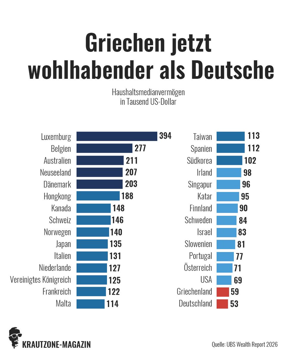
Sie reden immer nur über "das reiche Land", verschweigen aber, dass die Deutschen arm sind.

Und so bezahlt "das reiche Land" mit den armen Bürgern munter weiter an "die armen Länder" mit den reichen Bürgern.

Die armen Menschen bezahlen also das Leben der reichen Menschen. Genannt wird das EU.

Grafik: @KraZMagazin

[mr_atari @mr_atari77]

@ernsterjuenger Irgendwie bizarr.
Kannibalismus ist also kein Tabu. Es ist einfach nur schlecht für die Gesundheit. So wie Burger mit Pommes.

[mr_atari @mr_atari77]

Es gibt zahlreiche Beispiele, wo drastische Steuersenkungen erhebliche Mehreinnahmen an Steuern bedeuteten.
Russland unter Putin senkte die Unternehmenssteuer von 75% auf 25% -> Im selben Jahr doppelte Einnahmen

Auch die Steuerreform war genial: 10% Sozialabgaben pauschal. 10% Einkommenssteuer pauschal.
Das BIP verdoppelte sich innerhalb von ca 8 Jahren

[mr_atari @mr_atari77]

@Jaibee8Gee Normalverdiener zahlen knapp 50% + 19% MwSt

[mr_atari @mr_atari77]

@Jaibee8Gee In Deutschland zahlt ein Mindestlöhner 40% Steuern und Abgaben