harmonics

pharos

[harmonics @patternsonwaves]

@S_Conradi Hello

That is very nice

Do you have a public repository?

[Genes & Diseases Journal @GenesNDiseases]

This review explores the diverse functions of MFSD proteins and their emerging promise as therapeutic targets across human diseases.

[harmonics @patternsonwaves]

Wealth Is Not Money https://t.co/iylpQShZzh

[Pixel Symphony @Pixel0Symphony]

Archetypes, 2024.

[Probability and Statistics @probnstat]

Binomial Distribution:

[gozo @uncertaingaze]

⏳

[harmonics @patternsonwaves]

Endless Spiral of Little Men

Animation built on an Iterated Function System (IFS) from Michael Barnsley’s Fractals Everywhere.

#fractal #iteration #function #system #algorithm

[Brian @Inspector_9]

Waveforms of being • @poetengineer__

[Daniel Mentrard @dment37]

View of Divergence and Rotational(Curl) of a VectorField
Visualization |Animation | Interactive applet
@geogebra
https://t.co/s8R8SUoBzg
#geogebra #math #science #iteachmath #mtbos #visualization #elearning @bancoche #physics

[harmonics @patternsonwaves]

Most of so called intelligent systems of today are intelligent by stupidity of people

[Engineering Explained @Engineering67]

Visualize the tricky link between velocity and pressure.

[Water flowing | anbello.eth | anbello.tez @Waterflowing0]

In 2025, I started and, for various reasons, didn't finish several projects. I hope 2026 will be better for me and that I'll have the energy to finish them all (well, at least some). I wish the same for everyone: to be able to continue and hopefully complete their projects.

[this is one]

[Mathelirium @mathelirium]

Lecture 3 of our Quantum Mechanics series.

Lecture 2 gave us the one clean privilege quantum theory offers: treat ψ(x,t) as the state and ρ(x,t) = |ψ(x,t)|² as probability, because Schrödinger evolution forces ρ to obey a continuity equation. Lecture 3 is what that continuity equation is really telling you. If ρ behaves like a fluid, then the only question that matters is:

What is the velocity field?

Write

ψ(x,t) = r(x,t) exp(i θ(x,t)).

The magnitude r sets how much probability is sitting there. The phase θ sets where it tries to go. When you unpack the current j = Im(ψ* ∇ψ), it collapses to j = (ρ/m) ∇θ, which means the flow lines you draw are literally contours of phase geometry. Then the constraint that makes the picture bite: ψ has to be single-valued, so θ can’t wind by an arbitrary amount. Around any closed loop the total phase change must be 2π n, with n an integer. That’s why vortices aren’t features you add...they’re defects the math permits, in quantized units.

In the render you see both layers at once...the 3D surface shows |ψ| breathing while the phase skin slides, and the 2D panel exposes the engine...current lines steering around discrete vortex charges.

The math breakdown

We write the state as a complex field ψ(x,t) on the plane (x in R²). The Born rule defines the probability density

ρ(x,t) = |ψ(x,t)|²

Schrödinger evolution (ħ = 1 units) is

i ∂ψ/∂t = [ −(1/2m) ∇² + V(x,t) ] ψ

Now derive conservation of probability. Start with ρ = ψ*ψ:

∂ρ/∂t = ψ* (∂ψ/∂t) + ψ (∂ψ*/∂t)

Use Schrödinger and its complex conjugate:

∂ψ/∂t = (1/i) [ −(1/2m) ∇²ψ + Vψ ]
∂ψ*/∂t = (−1/i) [ −(1/2m) ∇²ψ* + Vψ* ]

Substitute. The V terms cancel, and the remaining terms rearrange into the continuity equation

∂ρ/∂t + ∇·j = 0

with probability current

j = (1/2mi) ( ψ* ∇ψ − ψ ∇ψ* )
= (1/m) Im(ψ* ∇ψ)

So "probability density" really behaves like a conserved fluid density with flux j.

Now expose the phase mechanism. Write ψ in polar form

ψ(x,t) = r(x,t) exp(i θ(x,t))

Compute the gradient

∇ψ = exp(iθ) (∇r + i r ∇θ)

Then

ψ* ∇ψ = r (∇r + i r ∇θ)

Taking the imaginary part gives

Im(ψ* ∇ψ) = r² ∇θ = ρ ∇θ

So the current becomes

j = (ρ/m) ∇θ

That’s the steering-wheel statement:

Phase gradient sets the flow direction and speed (modulated by density and m).

Finally, quantized vortices.

Because ψ must be single-valued, going around any closed loop must return the same complex value. That forces the phase winding to be an integer multiple of 2π:

∮ ∇θ · dl = 2π n with n in Z

n is the vortex charge. Vortex cores sit where ρ ≈ 0 (phase is undefined), and the current streamlines circulate around them.

#QuantumMechanics #Wavefunction #SchrodingerEquation #BornRule #ProbabilityCurrent #ContinuityEquation #Phase #Vortices #TopologicalDefects #ComplexAnalysis #MathematicalPhysics #Mathematics #Physics

[Simone Conradi @S_Conradi]

Each blob is an eigenvalue. At every frame, I apply small random perturbations and compute eigenvalues each time, this builds the blobs. A real parameter t drives the animation. Thanks to @reidatcheson for making me think about pseudospectra.
Made with #python #numpy #matplotlib

[Brian Roemmele @BrianRoemmele]

This is the work of neuroscientist Karl Pribram, "The Einstein of Brain Science," who challenged conventional understandings of the brain, perception, and reality itself.

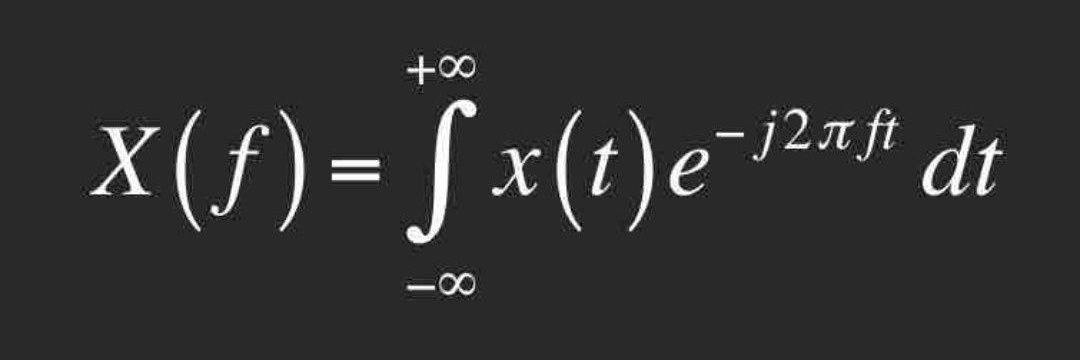
It shows intelligence and memory are Fourier transforms of waves for discernment and cognition.

It is key.

[MATLAB @MATLAB]

A tiny change can change everything.

The Lorenz system demonstrates the “butterfly effect,” where subtle differences in initial conditions lead to very different outcomes. This simulation visualizes that divergence across 10 starting points.

Check it out ⤵️ 🦋

[harmonics @patternsonwaves]

@mfranz_on Hi. Can you share the code?