Pawan Kumar Chahar

Data Engineer | Distributed System | Batch & Stream

#Bigdata #Python #Snowflake #dbt #PySpark #Docker #ApacheIceberg #GCP #AWS #Databricks

[Azalia Mirhoseini @Azaliamirh]

Bringing up the software stack for a new chip has always been a major bottleneck. That's about to change as we enter the era of AI as a compiler!

The model directly translates source code (e.g., Triton) to low-level assembly (e.g., PTX), and a verifier checks functional correctness through symbolic / numeric analysis, as well as other properties such as race conditions and deadlocks! No need for manually constructed layers of IR and DSLs.

Speedups over Triton baselines on B200:
FlashAttention (1.37x)
Mamba2 state forward (1.10x)

Great work led by @cos_francois, in collaboration with Charly Castes and Thomas Bourgeat from EPFL!

More to come soon!

[wafer @wafer_ai]

we gathered all the resources you'll ever need to become the most cracked ai performance engineer

follow and save to keep up with the series. links in thread 🧵

part 7: Efficiently Scaling Transformer Inference

Reiner Pope and coauthors studied PaLM inference on TPU v4. the paper gives performance engineers a way to reason about where weights, activations, and KV caches should live, what must move each step, and which transfers limit latency.

the paper's mechanisms suggest these checks for an inference deployment:

- prefill and decode can have different arithmetic intensity, meaning computation per byte transferred. prefill can process many prompt tokens in one pass; standard autoregressive decode produces one new token per sequence per step. larger decode batches amortize weight reads, but add sequence-specific KV cache traffic. sweep batch size with context length and profile the linear layers and attention to locate the bandwidth or compute limit.

- tensor parallelism can reduce local compute without removing the communication bottleneck. in the paper's 1D layout, activation-aggregation time stays roughly constant as chip count grows for a fixed workload. 2D partitioning splits both weight dimensions so each chip communicates smaller activation shards. evaluate this against the actual interconnect and matrix dimensions before increasing the parallelism degree.

- the best tensor to move changes with the token batch. weight-stationary layouts exchange activations; weight-gathered layouts transfer more weights to reduce activation exchange. large prefills can justify that trade because their activation tensors are large. count the tokens processed per forward pass, including prompt tokens during prefill, when comparing those layouts.

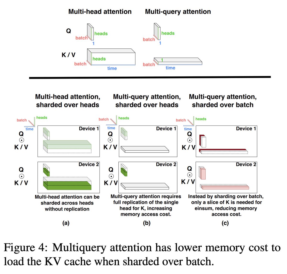
- multiquery attention shares one KV head across query heads, but a head-sharded layout can replicate that cache across devices. the paper shards attention across the batch during decode and exchanges current-step activations to reduce cache reads per chip. in vLLM's grouped-query attention deployments, check whether tensor parallelism exceeds the KV-head count and introduces cache replication before estimating per-GPU capacity.

- KV cache capacity and prefill attention intermediates are separate memory problems. at a fixed batch size and query-head count, sharing KV heads does not shrink the full attention-score tensor. for dense prefill, that tensor's element count grows with the square of sequence length. Appendix G discusses microbatching to reduce temporary allocations and FlashAttention to avoid materializing the full score matrix. use that distinction to identify whether a memory failure comes from retained KV state or temporary attention allocations.

- communication overlap depends on the execution schedule and tensor layout. the authors use Looped CollectiveEinsum to overlap collectives with matrix multiplication, including choosing output sharding that exposes overlap opportunities. inspect a GPU timeline for exposed communication and dependent compute stalls; an asynchronous collective does not establish that its cost is hidden.

- quantization changes different bottlenecks depending on what is quantized. the paper stores weights in int8 while retaining bfloat16 matrix arithmetic. this reduces weight-loading traffic, but does not provide faster arithmetic for compute-bound batches. evaluate weight, activation, and KV cache precision against the measured bottleneck and benchmark the effect on both phases.

- benchmark the operating point that the application needs. the paper compares latency with accelerator-time per token and model FLOPS utilization. in a serving system, track time to first token, inter-token latency, and throughput under the target load. keep queueing time separate from prefill time.

the practical use is to narrow an optimization experiment: estimate compute, HBM traffic, and collective costs for the actual workload, inspect the bottleneck, change the relevant layout or precision, and remeasure at the same latency target.

[Pawan Kumar Chahar @pavankumar123_]

@raila_san Good to see you all in one frame.

[Lummox @Lummox_eth]

Stanford put one of its most useful AI lectures online for free.

Andrew Ng and Kian Katanforoosh break down the architecture behind modern AI applications: prompting, RAG, and agents.

One example is almost absurd: a 20+ hour banking task can potentially be cut by 20–60% with an agentic workflow.

This is Lecture 8 of Stanford CS230, one of the university’s deep learning courses.

And the interesting part is how quickly the lecture moves beyond “just use a better model.”

The core idea is that the model is only one piece of the system.

A useful AI application can combine prompting with external context, retrieval, memory, tools, and multiple agents working on separate parts of the same problem.

Stanford shows this with a real enterprise workflow.

A financial institution may spend 1–4 weeks producing a single credit-risk memo.

The relationship manager gathers information from 15+ sources.

A credit analyst can then spend 20+ hours writing the memo.

It gets reviewed.

Feedback comes back.

Another draft gets written.

Now replace parts of that chain with agents.

One agent can break the project into tasks.

Specialized agents can gather information from different sources, analyze it, collaborate on a draft, then incorporate human feedback into the final version.

The estimate presented in Stanford’s material is a 20–60% reduction in the time spent creating these memos.

And that example explains the bigger point of the lecture.

The next generation of AI applications isn’t necessarily about asking one model a better question.

It’s about building a system around the model.

Prompts tell it what to do.

RAG gives it information it doesn’t already have.

Tools let it interact with external systems.

Agents let a larger objective become a sequence of smaller actions.

That’s the shift from using an LLM as a chatbot to using one as part of a workflow.

The lecture was taught at Stanford on November 11, 2025, as part of CS230, with Andrew Ng and Kian Katanforoosh listed as instructors. Stanford later published the recording publicly.

Almost 500,000 people have already watched it.

The entire lecture is still online for free.

[Dara @daraladje]

Should 100x AI Engineers be treated like elite athletes?

Kian Katanforoosh (@kiankatan) thinks your best engineer could get the Cristiano Ronaldo treatment: each supported by 3 culture architects whose only job is keeping them happy and performing.

At Workera, Kian is designing the future of workplace performance. Today we discuss:

03:50 - His AI course that taught 1M+ students

07:37 - Why we need AI mentors now

08:45 - Humans judging skill is unethical (maybe illegal)

13:06 - Success signs everyone overlooks

14:45 - The trap ambitious people keep falling into

16:02 - One metric that actually predicts success

17:08 - New jobs, and everything becomes pro sports

19:33 - How to adapt in the AI era

21:32 - The AI mentor Kian has to help you

[Tejas @taashuu_]

After co-working with @ankushdharkar, I realized

The difference between a junior and a senior engineer isn’t how often they fail.
It’s how many more times the senior engineer has already tried, failed, and learned.

[Puneet Patwari @system_monarch]

System design round at Databricks:

One customer query burned $180,000 of compute in 9 hours before anyone noticed.

The query was valid. The user had permissions. The cluster auto-scaled exactly as configured.

But some of your customers legitimately run $200,000 jobs, and for others a $2,000 job is a runaway accident.

The same query means different things depending on who ran it.

How do you build cost guardrails without asking every customer to define their own?

[Pawan Kumar Chahar @pavankumar123_]

@edinsoncode I am 8+ yrs exp Data Engineer experts in Building end to end Modern Data Warehouse use Databricks or Snowflake and AWS GCP Azure https://t.co/lKepBnPluz Metadata driven framework and Data Quality framework for Monitoring.

[Pawan Kumar Chahar @pavankumar123_]

People are working in Big Data or Data Engineering role Apache Spark realese 4.0 version which is support Declarative Framework to write all transformation with min code and make lineage graph in dependency. DQX framework is also helpful for data quality control.

[Abhishek Singh @0xlelouch_]

System design interview prompt: design Amazon order tracking (customer sees status + a timeline from purchase to delivered/returned).

Start by pinning requirements:
1) Read heavy. Tracking page refreshes a lot. Assume 50k req/s avg, 10x peak (sales events + delivery windows).
2) Write stream of events from many producers: checkout, warehouse, carrier webhooks, returns. 5k events/s, bursts, duplicates, out of order.
3) Latency: tracking page p95 < 200ms. Event ingestion can be async (seconds OK).
4) Correctness: never lose events. Customers must not see status go backwards.

APIs + data model:
1) GET /orders/{orderId}/tracking -> current_status + ordered timeline + last_updated
2) POST /tracking/events (internal) -> idempotent ingest: (orderId, eventId, source, type, ts, payload)
3) Core tables:
- orders(orderId, userId, createdAt, …)
- tracking_events(orderId, eventId, seq?, eventTime, receivedTime, type, payload)
- tracking_view(orderId, currentStatus, timelineJson, version, updatedAt)
4) Partition by orderId. eventId is unique per source for dedupe.

Architecture:
1) Producers publish events to Kafka/Kinesis. Keep raw event log for replay.
2) Stream processor builds a materialized view per orderId (tracking_view). This is what the read path hits.
3) Read path: API Gateway -> Tracking Service -> cache (Redis) -> tracking_view store (DynamoDB/Cassandra/Postgres partitioned).
4) Optional: push updates to UI via SSE/WebSocket, but polling is acceptable if cached.

Scaling choices + tradeoffs:
1) Materialized view avoids fan-out queries across many systems on every page load.
2) Keep raw events for audit/debug, but serve from tracking_view for speed.
3) Dynamo/Cassandra give easy partition scaling; Postgres works if sharded and you keep reads on an index by orderId.
4) Cache TTL small (5–30s). Invalidate on new event to cut staleness during active deliveries.

Ordering + state machine:
1) Define allowed transitions: Placed -> Packed -> Shipped -> OutForDelivery -> Delivered, plus exception paths.
2) Handle out-of-order by sorting on (eventTime, receivedTime) but never allow status regression.
3) If carrier timestamps are junk, use receivedTime for ordering and keep eventTime as display-only.

Failure cases to call out:
1) Duplicate webhooks: require idempotency key (eventId). Store seen ids per orderId window.
2) Missing events: tracking_view can be rebuilt from raw log. Run periodic reconciliation jobs.
3) Partial outage of stream processor: backlog grows, reads still work off last view; show last_updated and avoid lying.
4) Hot partitions (celebrity orders, batch updates): rate limit per orderId, use adaptive partitions or split by (orderId, shipmentId)
5) Data corruption: append-only raw log + versioned view lets you roll forward by replay, not manual edits

[Abhishek Singh @0xlelouch_]

Top 10 resources to learn Kafka + event-driven systems (practical for people shipping + on call):

1) Kafka docs (Quickstart + Concepts + Configs). The fastest way to learn what brokers, partitions, leaders, ISRs, and consumer groups actually do.

2) Confluent Developer site + tutorials. Clear writeups on keys, ordering, compaction vs retention, exactly-once semantics, Kafka Streams patterns.

3) Book: Kafka: The Definitive Guide. Good mental model for producers/consumers, partitioning, delivery semantics, and the knobs you’ll touch in prod.

4) Book: Designing Data-Intensive Applications (Kleppmann). The best source for the why: logs, stream processing, CDC, consistency tradeoffs.

5) Blog: Confluent blog (esp. performance + ops posts). Practical topics like rebalance pain, batching, idempotent producer, throughput vs latency.

6) Blog: Uber Engineering, LinkedIn Engineering, Netflix TechBlog posts on streaming. Real constraints: multi-region, schema governance, incident patterns.

7) Course: Confluent Fundamentals + Kafka Administration (or equivalent). Helps when you’re the one paging on partition under-replication at 2am.

8) Practice project: build an outbox + CDC pipeline (Postgres -> Debezium -> Kafka -> consumer). Forces you to learn idempotency, retries, dedupe, and replay.

9) Practice project: tiny order system with event versioning. Emit OrderCreated/Updated, evolve schemas, handle old events, and prove consumers don’t break.

10) Tooling: run a local stack with Docker Compose (Kafka + Schema Registry + Kafka UI) and do failure drills: kill a broker, add partitions, trigger a rebalance, measure lag in seconds not vibes

[generated using my AI agent, hope this was useful]

[Sunny R Gupta 🐰 @sunnykgupta]

I’m hiring a full-time UX Designer for @MetaformsAI

We’re a vertically integrated AI SaaS platform that helps market research teams execute real production work, from survey programming and QA to data validation and reporting.

The design challenge is making complex agentic workflows feel simple, while keeping humans firmly in control.

If you know a strong UX/Product Designer who’d be great at this, tag them below. If you don’t, repost anyway. Good karma, networking points, and a statistically unverified chance of your next coffee being free.

JD in the replies.

[Hendrix Liu @HendrixLiu29208]

we're hiring across the board (both in-person and remote), and except for a few roles, we don't care much about yoe

if you're high-agency and willing to put in the reps required to take a fast-paced early-stage startup from 1 to 10, that's p much all we need.

show me something you built: could be an interesting side project, a tool you made because you needed it, or something nobody assigned to you but you built it anyway.

anything that tells me almost everything i need to know about you in 5 mins while most profiles try to get past our ats

[Pawan Kumar Chahar @pavankumar123_]

Thrilled to receive the Stellar Performance Award at EXL!

Proud to have taken ownership as an IC on the Fintech Challenge project.

Grateful for the recognition!

[Sarvam @SarvamAI]

Introducing Saaras V4 Multi-speaker

Our best-in-class speech recognition model that accurately captures overlapping conversations and multi-speaker interactions, while delivering state-of-the-art performance in English across accents.

[The Offline Network @OfflineOnAir]

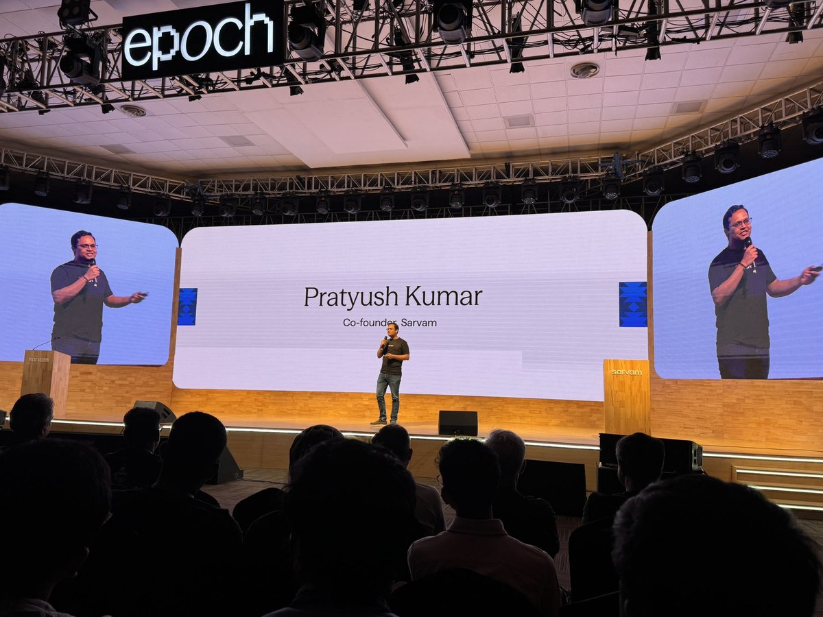
Everything Sarvam announced at Epoch:

MODELS
1/ Sarvam 105B (upgraded)
2/ Sarvam Vision 2.0: doc AI with native key-value extraction
3/ Saras V4 (speech-to-text): now SOTA on global English
4/ Saras V4 multi-speaker: transcribes people talking over each other
5/ Bulbul V4 (text-to-speech): one of India's most expressive TTS

INFRA
6/ Sarvam Inference: serves top open models from Indian soil
7/ Custom model training: your own model on Sarvam's infra
8/ Compute: now running the largest Blackwell cluster in India
9/ Opening a San Francisco office + bringing on Devendra Chaplot as advisor

PRODUCTS
10/ Voice Agents: build one in <60 min
11/ Work Agents: secure sandbox, Slack-native
12/ Content Studio: 50+ voices, voice cloning, motion-picture-grade dubbing
13/ Document Agents: extract, digitize & translate English and Indic
14/ Sarvam Code (beta): open-model coding harness

SOVEREIGN + DEVICES
15/ Chanakya: full on-prem stack built for defense & national security
16/ Kaze: AI-powered smart glasses
17/ Kivi: a voice dictation tool

[Tech Fusionist | Kushal Gangil @techyoutbe]

95% of Kubernetes Interviews Ask These 30 Concepts.
Are You Ready?

[Pawan Kumar Chahar @pavankumar123_]

@tiwarisuhani_11 Congratulations your all hard work and commitment

[Qiusheng Wu @giswqs]

GeoLibre v2.3.0 is here!

GeoLibre is a free and open-source, lightweight, cloud-native GIS platform for visualizing, exploring, and analyzing geospatial data. It runs everywhere you do, in the web browser, on the desktop, on mobile, and inside Jupyter notebooks, all while keeping your data local and private.

This release brings a legend that writes itself from your symbology, a new GeoLens catalog browser, and 200+ GeoLibre Rust geoprocessing tools running entirely in the browser.

What's new in v2.3.0

- Automatic on-map Legend: the legend builds itself from your visible layers, with class rows for graduated, categorized, rule-based, and expression styling, gradient bars for heatmaps and raster colormaps, and land-cover labels from a Raster Attribute Table. Rename, hide, reorder, or add your own entries, and it saves with the project.
- Symbology swatches in the Layers panel: every row shows a dot, line, square, or image glyph in the layer's own color, so a tall layer stack reads at a glance.
- GeoLens catalog browser: connect to a self-hosted GeoLens server, search its catalog, and add datasets as vector tiles, GeoJSON, or rendered raster tiles.
- Emerging Hot Spot Analysis: build a space-time cube from timestamped points and classify every cell as a new, intensifying, persistent, diminishing, sporadic, oscillating, or historical hot or cold spot, all client side.
- Mosaic time series: the Time Slider now steps through MosaicJSON and STAC collections of many COGs per date, on either a GPU or a WASM rendering engine.
- Copy and paste layer styles: give a whole set of layers one consistent look without restyling each in turn.
- Shareable tool links: deep-link any Whitebox tool with a ?tool= URL that opens the dialog preselected and pre-fills the form, with a Copy link button to build it for you.
- Smarter data loading: pick which layers to load from a multi-layer GeoPackage, import CSVs whose coordinates are in any projected CRS, and read a raster's real CRS, pixel size, and extent from the metadata dialog.
- Multiple AI profiles: define several provider, model, and credential setups, pick a default, and switch between them from the assistant panel.

Try it out

- Launch GeoLibre Web: https://t.co/8gMtkVtfnm
- GitHub: https://t.co/VXq8c1o2Nd
- Documentation: https://t.co/7VA2AQoCUc
- Release notes: https://t.co/cf3fXneeh6

#GIS #Geospatial #OpenSource #RemoteSensing #MapLibre #GeoLibre

[Tom Yeh @ProfTomYeh]

Vector Database by hand ✍️ ~ 10 steps walkthrough below

Vector databases are the backbone of Retrieval Augmented Generation (RAG).

How do they actually work?

Goal: index three sentences, then answer a query by finding the nearest one, filling in every cell yourself.

= 1. Given =

A dataset of three sentences, three words each. In practice it is millions of them.

= 2. Word embeddings =

Let us look up each word in an embedding table. Here the vocabulary is 22 words; in practice it is tens of thousands, and the vectors have thousands of dimensions rather than four.

= 3. Encoding =

We feed the sequence to an encoder, one linear layer and a ReLU, and get one feature vector per word. In practice the encoder is a transformer.

= 4. Mean pooling =

Let us average across the columns. Three word vectors collapse into one, which is what people mean by a text embedding or a sentence embedding.

= 5. Indexing =

We multiply by a projection matrix and the four dimensions become two. It is doing the job of a hash: a short representation that is faster to compare, and it is what gets saved in the vector storage.

= 6. Process "who are you" =

Let us repeat steps 2 to 5 on the second sentence.

= 7. Process "who am I" =

We do it a third time. The database is now indexed.

= 8. Query "am I you" =

Let us push the query through the very same pipeline: lookup, encoder, mean pooling, projection, and it lands as a 2D vector in the same space.

= 9. Dot products =

We transpose the query and multiply, which takes the dot product against every stored vector at once. The dot product is the estimate of similarity.

= 10. Nearest neighbour =

Let us scan for the largest: 60/9 beats 44/9 and 40/9, so the answer is "who am I". Scanning billions of vectors one at a time is what makes this the slow step in practice, which is why real databases use an approximate nearest neighbour index like HNSW.

The outputs:
Stored index vectors = [5/3, 2/3], [5/3, 0], [7/3, 2/3]
Query vector = [8/3, 2/3]
Dot products = 44/9, 40/9, 60/9
Nearest neighbour = "who am I"

The takeaway: a vector database is an embedding pipeline, a projection, and a dot product. Every step here is arithmetic you can do in pen, which is worth remembering when the word "database" makes it sound like something else.

💾 Save this post!