The Fisher Information Metric is a fundamental concept linking probability, statistics, and geometry. For a parametric model p(x;θ), it is defined as I(θ) = E[(∂/∂θ log p(x;θ))²], measuring how sensitive a distribution is to changes in θ. Geometrically, it induces a Riemannian metric on the space of probability distributions, forming the basis of information geometry. In statistics, it determines the Cramér–Rao lower bound, setting a limit on estimator variance. In machine learning, it appears in natural gradient descent, where updates are scaled by the inverse Fisher matrix, leading to more efficient optimization in deep models. In real life, it underpins signal processing, neuroscience (neural coding efficiency), and experimental design, where maximizing Fisher information ensures more informative data collection and better inference.
New lecture is live! 🌪️
What makes an attractor “strange”?
I define attractors and transitive attractors, then explore fractal structure through the solenoid attractor and inverse limit spaces. Symbolic dynamics returns in a new form.
🎥https://t.co/iwIdq7nAuu
Preprint: How Out-of-Equilibrium Phase Transitions can Seed Pattern Formation in Trained Diffusion Models
A synthesis of our work on symmetry bearking (ft @gaboraya) and @MasonKamb and @SuryaGanguli work on pattern formation from locality
Highly AI powered, many thanks to GPT!
Math, physics, chaos, cellular automata.
Free book. Introduces students to math/computational modeling in the interdisciplinary field of Complex Systems Science.
-Contents-
I Preliminaries
1 Introduction
1.1 Complex Systems in a Nutshell
1.2 Topical Clusters
2 Fundamentals of Modeling
2.1 Models in Science and Engineering
2.2 How to Create a Model
2.3 Modeling Complex Systems
2.4 What Are Good Models?
2.5 A Historical Perspective
II Systems with a Small Number of Variables
3 Basics of Dynamical Systems
3.1 What Are Dynamical Systems?
3.2 Phase Space
3.3 What Can We Learn?
4 Discrete-Time Models I: Modeling
4.1 Discrete-Time Models with Difference Equations
4.2 Classifications of Model Equations
4.3 Simulating Discrete-Time Models with One Variable
4.4 Simulating Discrete-Time Models with Multiple Variables
4.5 Building Your Own Model Equation
4.6 Building Your Own Model Equations with Multiple Variables
5 Discrete-Time Models II: Analysis
5.1 Finding Equilibrium Points
5.2 Phase Space Visualization of Continuous-State Discrete-Time Models
5.3 Cobweb Plots for One-Dimensional Iterative Maps
5.4 Graph-Based Phase Space Visualization of Discrete-State Discrete-Time Models
5.5 Variable Rescaling
5.6 Asymptotic Behavior of Discrete-Time Linear Dynamical Systems
5.7 Linear Stability Analysis of Discrete-Time Nonlinear Dynamical Systems
6 Continuous-Time Models I: Modeling
6.1 Continuous-Time Models with Differential Equations
6.2 Classifications of Model Equations
6.3 Connecting Continuous-Time Models with Discrete-Time Models
6.4 Simulating Continuous-Time Models
6.5 Building Your Own Model Equation
7 Continuous-Time Models II: Analysis
7.1 Finding Equilibrium Points
7.2 Phase Space Visualization
7.3 Variable Rescaling
7.4 Asymptotic Behavior of Continuous-Time Linear Dynamical Systems
7.5 Linear Stability Analysis of Nonlinear Dynamical Systems
8 Bifurcations
8.1 What Are Bifurcations?
8.2 Bifurcations in 1-D Continuous-Time Models
8.3 Hopf Bifurcations in 2-D Continuous-Time Models
8.4 Bifurcations in Discrete-Time Models
9 Chaos
9.1 Chaos in Discrete-Time Models
9.2 Characteristics of Chaos
9.3 Lyapunov Exponent
9.4 Chaos in Continuous-Time Models
III Systems with a Large Number of Variables
10 Interactive Simulation of Complex Systems
10.1 Simulation of Systems with a Large Number of Variables
10.2 Interactive Simulation with PyCX
10.3 Interactive Parameter Control in PyCX
10.4 Simulation without PyCX
11 Cellular Automata I: Modeling
11.1 Definition of Cellular Automata
11.2 Examples of Simple Binary Cellular Automata Rules
11.3 Simulating Cellular Automata
11.4 Extensions of Cellular Automata
11.5 Examples of Biological Cellular Automata Models
12 Cellular Automata II: Analysis
12.1 Sizes of Rule Space and Phase Space
12.2 Phase Space Visualization
12.3 Mean-Field Approximation
12.4 Renormalization Group Analysis to Predict Percolation Thresholds
13 Continuous Field Models I: Modeling
13.1 Continuous Field Models with Partial Differential Equations
13.2 Fundamentals of Vector Calculus
13.3 Visualizing Two-Dimensional Scalar and Vector Fields
13.4 Modeling Spatial Movement
13.5 Simulation of Continuous Field Models
13.6 Reaction-Diffusion Systems
14 Continuous Field Models II: Analysis
14.1 Finding Equilibrium States
14.2 Variable Rescaling
14.3 Linear Stability Analysis of Continuous Field Models
14.4 Linear Stability Analysis of Reaction-Diffusion Systems
15 Basics of Networks
15.1 Network Models
15.2 Terminologies of Graph Theory
15.3 Constructing Network Models with NetworkX
15.4 Visualizing Networks with NetworkX
15.5 Importing/Exporting Network Data
15.6 Generating Random Graphs
16 Dynamical Networks I: Modeling
16.1 Dynamical Network Models
16.2 Simulating Dynamics on Networks
16.3 Simulating Dynamics of Networks
16.4 Simulating Adaptive Networks
17 Dynamical Networks II: Analysis of Network Topologies
17.1 Network Size, Density, and Percolation
17.2 Shortest Path Length
17.3 Centralities and Coreness
17.4 Clustering
17.5 Degree Distribution
17.6 Assortativity
17.7 Community Structure and Modularity
18 Dynamical Networks III: Analysis of Network Dynamics
18.1 Dynamics of Continuous-State Networks
18.2 Diffusion on Networks
18.3 Synchronizability
18.4 Mean-Field Approximation of Discrete-State Networks
18.5 Mean-Field Approximation on Random Networks
18.6 Mean-Field Approximation on Scale-Free Networks
19 Agent-Based Models
19.1 What Are Agent-Based Models?
19.2 Building an Agent-Based Model
19.3 Agent-Environment Interaction
19.4 Ecological and Evolutionary Models
Bibliography
Index
Link: https://t.co/4Tjtn0L6JU
the difference between a biological neuron and an artificial neuron is massive.
they share the idea. not the reality.
what a biological neuron does:
• receives signals through dendrites → thousands of inputs, not just a few
• integrates over time → signals accumulate, decay, interact
• fires spikes → discrete events, not smooth numbers
• adapts continuously → plasticity rewires connections based on experience
• runs on chemistry + electricity → noisy, slow, but incredibly efficient
what an artificial neuron does:
• takes weighted inputs → simple numbers in, number out
• applies an activation function → relu, sigmoid, etc
• updates via backprop → global optimization, not local biology
• runs on silicon → fast, precise, but power-hungry
• no real “memory” → unless explicitly designed (rnn, transformers)
why it matters:
• ai today is inspired by the brain, not a replica of it.
• biological neurons are dynamic, adaptive, and energy-efficient.
• artificial neurons are simplified, scalable, and mathematically convenient.
we’re not building brains.
we’re building approximations that work well enough to be useful.
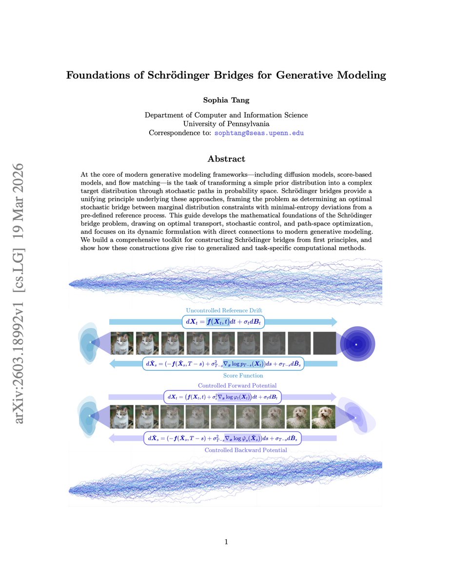
New tutorial paper on the “Foundations of Schrödinger Bridges for Generative Modeling” is out on arXiv! 🧩
📖 arXiv: https://t.co/ce4feGdXZT
🔮 Project Website: https://t.co/dyNr5TRijq
With 220 pages and 24 figures, this guide builds the theoretical foundations of Schrödinger bridges from the ground up, unifying the broad field of generative modeling with a single guiding principle: construct an optimal stochastic bridge between distributions while minimizing deviation from a reference process.
The rapid progress in generative modeling has made the field increasingly difficult to navigate from a foundational perspective, which motivated me to develop a resource that builds the core concepts needed to understand and contribute to new advances.
This guide contains intuitive explanations and step-by-step proofs covering:
🧩 The dynamic Schrödinger bridge formulation, lifting optimal transport to continuous-time stochastic processes between distributions, with direct connections to diffusion models, score-based methods, and flow matching.
🧩 A comprehensive toolkit for constructing Schrödinger bridges from first principles, describing stochastic optimal control, forward–backward SDEs, Doob’s h-transform, and Markov and reciprocal projections.
🧩 Extensions to complex and real-world problem settings, including the multi-marginal, unbalanced, discrete SB problems, highlighting the flexibility of the Schrödinger bridge framework in describing complex dynamical systems.
🧩 Practical, scalable algorithms for training and inference of dynamic Schrödinger bridges across modern generative modeling tasks.
More details in the thread 👇🏻
El artículo propone que los sistemas biológicos parecen más inteligentes que la IA actual porque distribuyen la adaptación en múltiples niveles de organización, desde células hasta organismos.
En cambio, en la mayoría de los sistemas de IA actuales la adaptación se concentra en las capas de software, mientras que las capas inferiores, como el hardware, permanecen fijas, lo que limita la capacidad de adaptación de los niveles superiores.
Utilizando Stack Theory, el autor demuestra matemáticamente que la capacidad de adaptación en un nivel depende de la flexibilidad de los niveles inferiores, formulado como The Law of the Stack.
Por tanto, si se quiere construir sistemas de IA más robustos y adaptativos, es necesario delegar la capacidad de adaptación hacia capas más profundas del sistema en lugar de centralizarla únicamente en una capa superior.
https://t.co/H8hIW88SYd
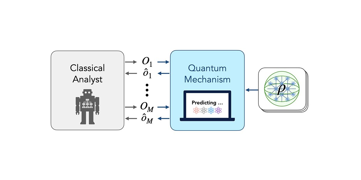
Fundamental limits of adaptive measurement in quantum many-body systems are established, showing when logarithmic-sample prediction fails and how optimal algorithms can still be achieved.
Read the paper: https://t.co/xQmSAesW7l
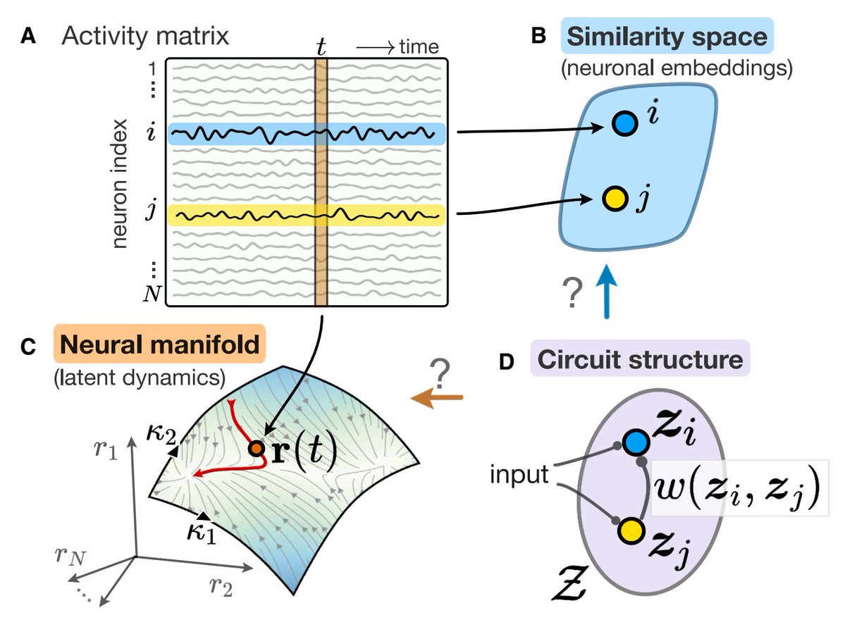
𝗪𝗵𝗮𝘁'𝘀 𝘁𝗵𝗲 𝗿𝗲𝗹𝗮𝘁𝗶𝗼𝗻𝘀𝗵𝗶𝗽 𝗯𝗲𝘁𝘄𝗲𝗲𝗻 𝗺𝗮𝗻𝗶𝗳𝗼𝗹𝗱𝘀 𝗮𝗻𝗱 𝗿𝗲𝗰𝘂𝗿𝗿𝗲𝗻𝘁 𝗻𝗲𝘁𝘄𝗼𝗿𝗸𝘀 𝗶𝗻 𝘁𝗵𝗲 𝗯𝗿𝗮𝗶𝗻?
This looks like a must read (suppl material bursting with goodies).
https://t.co/aMNOr9ReQV


![QuantumPapers's tweet photo. Tensor network influence functionals for open quantum systems with general Gaussian bosonic baths
Valentin Link
https://t.co/mkrxL3yVrD [𝚚𝚞𝚊𝚗𝚝-𝚙𝚑] https://t.co/6ledmRp6d2](https://pbs.twimg.com/media/HEPUXK3agAAY2oH.png)
![probnstat's tweet photo. The Fisher Information Metric is a fundamental concept linking probability, statistics, and geometry. For a parametric model p(x;θ), it is defined as I(θ) = E[(∂/∂θ log p(x;θ))²], measuring how sensitive a distribution is to changes in θ. Geometrically, it induces a Riemannian metric on the space of probability distributions, forming the basis of information geometry. In statistics, it determines the Cramér–Rao lower bound, setting a limit on estimator variance. In machine learning, it appears in natural gradient descent, where updates are scaled by the inverse Fisher matrix, leading to more efficient optimization in deep models. In real life, it underpins signal processing, neuroscience (neural coding efficiency), and experimental design, where maximizing Fisher information ensures more informative data collection and better inference.](https://pbs.twimg.com/media/HEJ8sY7WoAAG27R.jpg)


![QuantumPapers's tweet photo. Mixed-State Entanglement in a Minimal Model of Quantum Chaos
Tanay Pathak
https://t.co/U6QUrr874l [𝚚𝚞𝚊𝚗𝚝-𝚙𝚑 𝚌𝚘𝚗𝚍-𝚖𝚊𝚝.𝚜𝚝𝚊𝚝-𝚖𝚎𝚌𝚑 𝚑𝚎𝚙-𝚝𝚑] https://t.co/L1lg7ej5Ee](https://pbs.twimg.com/media/HDp0UATXcAAEYT7.png)