Ke.dev

independent developer | I ship. I iterate. I learn.

[Ke.dev @yangke687]

CS230 (2018) DL | Lecture 2
https://t.co/xjGS6Nvv60

📎 Softmax
Softmax is a mathematical function, typically used as an activation function in the very last layer of a neural network for multi-class classification tasks.

The main job is to turn raw, unformatted numbers into normalized probability distributions that sum up to exactly 100%.

Imagine that you pass an image into a neural network to identify whether it is a cat, a dog, or a bird.

1⃣: The raw network output
Before the softmax layer, the network outputs raw, unconstrained scores for each class. In ML, these scores are called Logits. They can be any real numbers. (positive, negative, large, or small)
Cat score: 2.0
Dog score: 1.0
Bird score: 0.1
These scores are hard to interpret. Does 2.0 mean 20%, 200%, or something else? We need Softmax to translate them into probabilities.

2⃣: The Softmax Transformation
The softmax function processes these logits in two distinct sub-steps:

2.1 Exponentiation
We raise the natural base e (2.718) to the power of each score: exp(score). This ensures all scores become strictly positive.

Cat: exp(2.0) ≈ 7.39
Dog: exp(1.0) ≈ 2.72
Bird: exp(0.1) ≈ 1.11
Sum of all exponents: 11.22

2.2 Normalization
We divide each individual exponent value by the total sum. This squeezes the final numbers into a range between 0 and 1:

Cat Probability: 7.39 / 11.22 ≈ 0.66 (66%)
Dog Probability: 2.72 / 11.22 ≈ 0.24 (24%)
Bird Probability: 1.11 / 11.22 ≈ 0.10 (10%)

3⃣ The Final Result
After Softmax, the network gives a clear, probabilistic output array: [0.66, 0.24, 0.10].
Now, the system can confidently say: "There is a 66% chance that this image is a cat." Because these are clean percentages, we can easily feed them into a Loss Function (like Cross-Entropy Loss) to calculate errors and help the network learn through backpropagation.

[Ke.dev @yangke687]

Committed all the problem set coding solutions and pushed them to:
https://t.co/f1enxbP5KR

[Ke.dev @yangke687]

CS229 (2018) Problem set #4

❓6-a:
Inverted Pendulum (Cart-pole) MDP Control Task

1. Task & Goal
The objective is to automatically design a control policy for an inverted pendulum (cart-pole) system without prior knowledge of the underlying physical dynamics. The system consists of a pole attached to a cart via a free-joint, with the cart moving along a frictionless, bounded track. Failure occurs if the pole angle deviates too far from the vertical or if the cart moves off the track edges. The goal is to apply horizontal forces to the cart to keep the pole balanced.

2. State & Action Spaces
The environment operates in discrete time-steps. The true system configuration is fully captured by a continuous 4-D state vector: cart position (x), cart velocity (ẋ), pole angle (θ), and pole angular velocity (θ̇). To simplify learning, the continuous space is discretized into a single integer ranging from 0 to NUM_STATES-1. At each step, the controller must choose exactly one of two actions: push the cart right (Action 0) or push the cart left (Action 1).

3. Reward & Transition Dynamics
The reward function R(s) depends solely on the current state. Safe balancing steps yield a reward of zero, while a negative reward (penalty) is triggered upon failure, which also prompts a random re-initialization. Although the underlying continuous physics are deterministic, the transition dynamics become non-deterministic in the discretized state space due to multiple continuous states mapping to the same discrete state.

4. Implementation: Model-based Reinforcement LearningInstead of model-free methods, the solution requires learning the MDP model explicitly from observed online data. The implementation steps are:Initialization:

4.1
Initialize all state rewards to 0 and all transition probabilities to a uniform distribution.

4.2
Online Data Collection: Accumulate counts of state transitions P(s'|s,a) and rewards during simulations.

4.3
Periodical Updates: To optimize efficiency, re-estimate the transition probabilities and rewards only when the cart fails.Value Iteration: Following each model update, solve Bellman's equations using Value Iteration (with a discount factor γ = 0.995) until the maximum absolute change in the value function falls below a pre-set tolerance.

4.4
Global Convergence: The overall learning process is deemed to have converged when the Value Iteration loop terminates in its very first iteration over multiple consecutive trials.

[Ke.dev @yangke687]

❓ 5-b: We say that V is a fixed point of B if B(V)=V. Using the fact that the Bellman update operator is a γ-contraction in the max-norm, prove that B has at most one fixed point, i.e., that there is at most one solution to the Bellman equations. You may assume that B has at least one fixed point.

📝Assume there are two fixed points, V_1 and V_2, such that
|| V_1 - V_2 ||∞ > 0
B(V_1) = V_1
B(V_2) = V_2

Bring them back to the conclusion of ❓5-a

|| B(V_1) - B(V_2 ||∞ ≤ γ || V_1 - V_2 ||∞

<=>

|| V_1 - V_2 ||∞ ≤ γ || V_1 - V_2 ||∞

=> 1 ≤ γ

But the problem statement tells us
the discount factor γ < 1.

So 1 ≤ γ is impossible!

[Ke.dev @yangke687]

CS229 Problem set question 4

Markov decision process
Consider an MDP with finite state and action spaces, and a discount factor γ < 1. Let B be the Bellman update operator, with V a vector of values for each state. I.e., if
V' = B(V), then

V'(s) = R(s) + γ max_a{a ∈ A} Σ_s'{s' ∈ S} P_sa(s')V(s')

❓5-a: Prove that, for any two finite value vectors V_1 and V_2, it holds true that

|| B(V_1) - B(V_2) ||∞ ≤ γ || V_1 - V_2 ||∞

where: ||V||∞ = max_{s ∈ S} |V(s)|

📝 Prove the max operator inequality for absolute value
1⃣
f(a) = f(a) - g(a) + g(a)
f(a) - g(a) ≤ | f(a) - g(a) | ≤ max_a' | f(a') - g(a') |

=> f(a) = f(a) - g(a) + g(a)
≤ max_a' | f(a') - g(a') | + g(a)
≤ max_a' | f(a') - g(a') | + max_a' g(a')

Consider the right-hand side part as a constant; any value of the function f(a) will be less than it

=> max_a' f(a') ≤ max_a' | f(a') - g(a') | + max_a' g(a')
=> max_a' f(a') - max_a' g(a') ≤ max_a' | f(a') - g(a') |

2⃣
g(a) = g(a) - f(a) + f(a)
g(a) - f(a) ≤ | g(a) - f(a) | ≤ max_a' |g(a') - f(a') |

=> g(a) = g(a) - f(a) + f(a)
≤ max_a' |g(a') - f(a') | + f(a)
≤ max_a' |g(a') - f(a') | + max_a' f(a')

=> max_a' g(a') ≤ max_a' |g(a') - f(a') | + max_a' f(a')
=> -max_a' |g(a') - f(a')| ≤ max_a' f(a') - max_a' g(a')
=> -max_a' |f(a') - g(a')| ≤ max_a' f(a') - max_a' g(a')

So, we have:
max_a' |g(a') - f(a') |
≥ max_a' f(a') - max_a' g(a')
≥ -max_a' |f(a') - g(a')|

According to if: -M ≤ X ≤ M, then X ≤ |M|

=> | max_a f(a) - max_a g(a) | ≤ max_a | f(a) - f(a) |

3⃣
Given:
B(V_1) = R(s) + γ max_a{a ∈ A} Σ_s'{s' ∈ S} P_sa(s') V_1(s')
B(V_2) = R(s) + γ max_a{a ∈ A} Σ_s'{s' ∈ S} P_sa(s') V_2(s')

Then:
| B(V_1) - B(V_2) | =
γ | max_a Σ_s' P_sa(s')V_1(s') - max_a Σ_s' P_sa(s')V_2(s')|
≤ γ max_a | Σ_s' P_sa(s')V_1(s') - Σ_s' P_sa(s')V_2(s') |
= γ max_a | Σ_s' P_sa(s') [ V_1(s') - V_2(s') ] |

according to: | x_1 + x_2 + ... + x_n | ≤ |x_1| + |x_2| + ... |x_n|

≤ γ max_a Σ_s' P_sa(s') | V_1(s') - V_2(s') |

According to the definition of the infinite norm
|| V_1 - V_2 ||∞ = max_s'{s' ∈ S} | V_1(s') - V_2(s') |
It does mean for any state s', | V_1(s') - V_2(s') | must be less than || V_1 - V_2 ||∞.

|B(V_1) - B(V_2)| ≤ γ max_a | Σ_s' P_sa(s') [ V_1(s') - V_2(s') ] |
≤ γ max_a Σ_s' P_sa(s') || V_1 - V_2 ||∞
ignore action a, and Σ_s' P_sa(s') = 1
= γ || V_1 - V_2 ||∞

For any state, the above inequality is established.

=> max_s{s ∈ S} |B(V_1) - B(V_2)| ≤ γ || V_1 - V_2 ||∞
=> || B(V_1) - B(V_2 ||∞ ≤ γ || V_1 - V_2 ||∞

[Ke.dev @yangke687]

❓4-c: Cocktail Party Problem
For this question, you will implement the Bell and Sejnowski ICA algorithm, but assuming a Laplace source (as derived in part-b), instead ,of the Logistic distribution covered in class. The file mix.dat contains the input data which consists of a matrix with 5 columns, with each column corresponding to one of the mixed signals x_i​. The code for this question can be found in p04_ica.py.
Implement the update_W and unmix functions in p04_ica.py.

You can then run p04_ica.py to split the mixed audio into its components. The mixed audio tracks are written to midex_i.wav in the output folder. The split audio tracks are written to split_i.wav in the output folder.

[Ke.dev @yangke687]

CS229 (2018) Problem set Question 4

❓4-a: We assume sources are distributed according to a standard normal distribution, i.e

s_j ~ N(0, 1)
j = {1, 2, ... d}

The likelihood of our unmixing matrix is:

ℓ(W) = Σ_i {i=1 to n}
[ log|W| + Σ_j {j=1 to d} log g'(w_j.T x_i) ]

where g is the cumulative distribution function (CDF), and g' is the probability density function (PDF) of the source distribution. Whereas in the notes we derive an update rule to train W iteratively, for the cause of Gaussian-distributed sources, we can analytically reason about the resulting W.

Try to derive a closed-form expression for W in terms of X when g is the standard normal CDF. Deduce the relation between W and X in the simplest terms, and highlight the ambiguity (in terms of rotational invariance) in computing W

📝 1⃣ g is CDF; g' is PDF
=> g'(w_j.T x_i) = 1/[(2π)^(1/2)] exp[ -1/2 (w_j.T x_i)^2 ]
=> log g'(w_j.T x_) = log 1/[(2π)^(1/2)] - 1/2 [(w_j.T x_i)^2]

ℓ(W) = nlog|W| + nd log 1/[(2π)^(1/2)]
- 1/2 Σ_j {j=1 to d} Σ_j {j=1 to d} [(w_j.T x_i)^2]

Drop the part that has no relation with W

ℓ(W) = nlog|W|
- 1/2 Σ_j {j=1 to d} Σ_j {j=1 to d} [(w_j.T x_i)^2]

where: x_i is a column vector
w_j is a column vector
w_j.T x_i is a scalar

2⃣According to the F-norm definition:
Σ_j {j=1 to d} Σ_j {j=1 to d} [(w_j.T x_i)^2]
= ||WX||_F^2
= Tr[ (WX) (WX).T ]
= Tr [ WX (X.T)(W.T) ]
Let X(X.T) = Σx (covariance matrix)
= Tr [ W Σx W.T ]

ℓ(W) = nlog|W| - 1/2 Tr [ W Σx W.T ]

3⃣ Take the derivative of ℓ(W) w.r.t W, and let it be 0

dℓ(W)/dW = n(W^-1).T - WΣx = 0
=> n(W^-1).T = WΣx
=> n(W^-1) = Σx.T W.T
=> n I = W Σx.T W.T
=> W (1/n Σx.T) W.T = I
=> the simplest closed-form: W Σx.T W.T = I

If W_0 is a specific solution to the whitening equation:
W Σx.T W.T = I, multiplying it by any arbitrary orthogonal rotation matrix R (R R^T = I) yields another valid solution W = RW_0

W Σx.T W.T = RW_0 Σx.T (RW_0).T
= RW_0 Σx.T W_0.T R.T
= R (W_0 Σx.T W_0.T) R.T
= I

that satisfies the same equation.

Consequently, for Gaussian sources, ICA can only recover the original signals up to an arbitrary rotation, making it impossible to uniquely determine the true independent sources.

[Ke.dev @yangke687]

❓4-b: We assume sources are distributed according to the standard Laplace distribution, i.e s_i ~ ℒ(0, 1). The Laplace distribution ℒ(0, 1) has PDF

f_ℒ(s) = 1/2 exp(-|s|)

With this assumption, derive the update rule for a single example in the form

W := W + α(...)

📝 For a single example x, x = [x_1, x_2, ... x_d]

ℓ(W) = log |W| + Σ_j {j=1 to d} log f_ℒ(w_j.T x)
= log |W| + Σ_j {j=1 to d} log [ 1/2 exp(- |w_j.T x| ) ]
= log |W| + Σ_j {j=1 to d} log(1/2) - | w_j.T x |
Drop the part that has no relation to W
= log |W| - Σ_j {j=1 to d} |w_j.T x|

1⃣ ∂(log|W|) / ∂W = (W^-1).T

2⃣ ∂( |w_j.T x| ) / ∂w_j = sign(w_j.T x) · x
∂( Σ_j {j=1 to d} |w_j.T x| ) / ∂W = sign(Wx) · (x.T)

=> ∂ℓ(W) / ∂W = (W^-1).T - sign(Wx) · (x.T)
=> W := W + α [ (W^-1).T - sign(Wx) · (x.T) ]

[Ke.dev @yangke687]

CS229 (2018) Problem set Question 4

Suppose we are given a set of points {x_1, x_2, ... x_m}. Let us assume that we have as usual preprocessed the data to have zero mean and unit variance in each coordinate. For a given unit-length vector u, let f_u(x) be the projection of point x onto the direction given by u. I.e, if V = {αu : α ∈ R}, then

f_u(x) = arg min_v∈V ( || x - v ||_L2 )^2

❓3-a:
Show that the unit-length vector u that minimizes the mean squared error between the projected point and the original points corresponds to the first principal component for the data. I.e, show that

arg min_u {u.T·u=1} Σ_i {i=1 to m} ( || x_i - f_u(x_i) ||_L2 )^2

(L2 norm)

gives the first principal component.

📝 1⃣ because v=αu
Let J(α) = ( || x - αu ||_L2 )^2
= (x - αu).T (x - αu)
= (x.T - αu.T) (x - αu)
= (x.T)x - α(x.T)u - α(u.T)x + (α^2) (u.T)u
(x.T)u is constant, ((x.T)u).T = (x.T)u = (u.T)x
= (x.T)x - 2α (u.T)x + (α^2) (u.T)u
= (x.T)x - 2α (u.T)x + (a^2)

Take the derivative of J(α) w.r.t α:
dJ(α)/dα = -2(u.T)x + 2α

Let it be 0:
-2(u.T)x + 2α = 0 => α = (u.T)x

it means the optimal α* = (u.T)x
the optimal v* = α*u = (u.T)xu

f_u(x) = arg min_v∈V ( || x - v ||_L2 )^2
= [(u.T)x]u

2⃣ Let
J(u) = Σ_i {i=1 to m} ( || x_i - f_u(x_i) ||_L2 )^2

( || x_i - f_u(x_i) ||_L2 )^2
= {x_i - [(u.T)(x_i)]u}.T { x_i - [(u.T)(x_i)]u }
= { (x_i).T - (u.T)[(u.T)(x_i)].T } { x_i - [(u.T)(x_i)]u }
= (x_i.T)(x_i)
- (x_i.T) [(u.T)(x_i)] u
- (u.T) [ (u.T)(x_i) ].T (x_i)
+ (u.T) [ (u.T)(x_i) ].T [(u.T)(x_i)] u
(u.T)(x_i) is constant, [ (u.T)(x_i) ].T = [ (u.T)(x_i) ]
= (x_i.T)(x_i)
- (x_i.T) [(u.T)(x_i)] u
- [ (u.T)(x_i) ] (u.T) (x_i)
+ [ (u.T)(x_i) ]^2
= (x_i.T)(x_i) - 2 [(u.T)(x_i)]^2 + [ (u.T)(x_i) ]^2
= (x_i.T)(x_i) - [(u.T)(x_i)]^2

=>
( || x_i - f_u(x_i) ||_L2 )^2 = (|| x_i ||_L2)^2 - [(u.T)(x_i)]^2

=>
J(u) = Σ_i {i=1 to m} (|| x_i ||_L2)^2 - [(u.T)(x_i)]^2
= Σ_i {i=1 to m} (|| x_i ||_L2)^2
-
Σ_i {i=1 to m} [(u.T)(x_i)]^2

The first part:
Σ_i {i=1 to m} (|| x_i ||_L2)^2
is a constant

The second part:
Σ_i {i=1 to m} [(u.T)(x_i)]^2
= Σ_i {i=1 to m} (u.T)(x_i)(u.T)(x_i)
= Σ_i {i=1 to m} (u.T)(x_i)(x_i.T)u
= (u.T) [Σ_i {i=1 to m} (x_i) (x_i.T)] u
covariance matrix Σ = 1/m Σ_i {i=1 to m} (x_i) (x_i.T)
= m (u.T) Σ u

After all these:
J(u) = Σ_i {i=1 to m} (|| x_i ||_L2)^2 - m (u.T) Σ u

arg min_u {u.T·u=1} J(u)
be equivalent to
arg max_u {u.T·u=1} u.T) Σ u

[Ke.dev @yangke687]

❓2-e: We will now consider several situations where you might have a choice between the importance sampling estimator and the regression estimator. Please state whether the importance sampling estimator or the regression estimator would probably work best in each situation and explain why it would work better. In all of these situations, your states ss consist of patients, your actions aa represent the drugs to give to certain patients, and your R(s, a) is the lifespan of the patient after receiving the drug.

i. Drugs are randomly assigned to patients, but the interaction between the drug, patient, and lifespan is very complicated.

📝π_0 is easy, so we choose Importance sampling.

ii. Drugs are assigned to patients in a very complicated manner, but the interaction between the drug, patient, and lifespan is very simple.

📝 π_0 is complicated but R(s,a) is simple, we choose Regression.

[Ke.dev @yangke687]

CS229 (2018) Problem Set Question 4

Most of the methods we discuss apply to general MDPs, but for the sake of this problem, we will consider MDP's with a single timestep. We consider a universe consisting of states 's', actions 'a', and a reward function R(s, a), where 's' is a state and 'a' is an action. One important factor is that we often only have a subset of 'a' in our dataset. For example, each state 's' could represent a patient, each action 'a' could represent which drug we prescribe to that patient, and R(s, a) could be their lifespan after prescribing that drug.

A policy is defined by a function π_i(s, a)=p(a∣s,π_i). In other words, π_i(s, a) is the conditional probability of an action given a certain state and a policy.

We are given an observational dataset consisting of
(s, a, R(s, a)) tuples.

Let p(s) denote the probability density function for the distribution of state s values within that dataset. Let π_0(s, a)=p(a∣s) within our observational data. π_0 corresponds to the baseline policy present in our observational data. Going back to the patient example, p(s) would be the probability of seeing a particular patient 's' and π_0(s, a) would be the probability of a patient receiving a drug in the observational data.

We are also given a target policy π_1(s, a), which gives the conditional probability p(a∣s) in our optimal policy that we hope to evaluate. One particular note is that even though this is a distribution, many of the policies that we hope to evaluate are deterministic, such that given a particular state s_i​, p(a∣s_i)=1 for a single action and p(a∣s)=0 for the other actions.

Our goal is to compute the expected value of R(s, a) in the same population as our observational data, but with a policy of π_1​ instead of π_0​. In other words, we are trying to compute:

E {s∼p(s); a∼π_1​(s,a)} ​​[ R(s,a) ]

Important Note About Notation And Simplifying Assumptions:

We haven’t really covered expected values over multiple variables such as

E {s∼p(s); a∼π_1(s, a)} [ R(s, a) ]

in class yet.

For purposes of this question, you may make the simplifying assumption that our states and actions are discrete distributions. This expected value over multiple variables simply indicates that we are taking the expected value over the joint pair (s, a) where 's' comes from p(s) and 'a' comes from π_1(s, a). In other words, you have a p(s, a) term, which is the probability of observing that pair, and we can factorize that probability to p(s)p(a∣s)=p(s)π1(s, a). In math notation, this can be written as:

E {s∼p(s); a∼π1​(s,a)​​ } [ R(s,a) ]
​=∑_s_a ​R(s,a) p(s,a)
=∑​_s_a R(s,a) p(s)p(a∣s)
=∑​_s_a R(s,a) p(s)π_1​(s,a)​

Unfortunately, we cannot estimate this directly as we only have samples created under policy π_0​ and not π_1​. For this problem, we will be looking at formulas that approximate this value using expectations under π_0​ that we can actually estimate.

We will make one additional assumption that each action has a non-zero probability in the observed policy π_0(s, a). In other words, for all actions 'a' and states 's', π_0(s, a) > 0.

Regression:
The simplest possible estimator is to directly use our learned MDP parameters to estimate our goal. This is usually called the regression estimator. While training our MDP, we learn an estimator Ŕ(s, a) that estimates R(s, a). We can now directly estimate

E {s∼p(s); a∼π_1(s,a)} [ R(s,a) ]
with
E {s∼p(s); a∼π_1(s,a)} [ Ŕ(s, a) ]

If Ŕ(s, a)=R(s, a), then this estimator is trivially correct.

We will now consider alternative approaches and explore why you might use one estimator over another.

❓2-a: Importance Sampling: One commonly used estimator is known as the importance sampling estimator. Let π̂_0​ be an estimate of the true π_0​. The importance sampling estimator uses π̂_0​ and has the form:

E {s∼p(s); a∼π_0(s, a)​​} [ π_1​(s, a) / π̂_0​(s, a) ​R(s, a) ]

Please show that if π̂_0=π_0​, then the importance sampling estimator is equal to:

E {s∼p(s); a∼π_1​(s,a)} [​ ​R(s,a) ]

📝 According to the expected value definition:
E {s∼p(s); a∼π_0(s, a)​​} [ π_1​(s, a) / π̂_0​(s, a) ​R(s, a) ]
= ∑​_s_a p(s, a) [ π_1​(s, a) / ​π̂_0​(s, a) ​R(s, a) ]
= ∑​_s_a p(s) π_0​(s, a) [ π_1​(s, a) / π_0​(s, a) ​R(s, a) ]
= ∑​_s_a p(s) π_1​(s, a) ​R(s, a)
= ∑​_s_a p(s) p​(a|s, π_1) ​R(s, a)
= ∑​_s_a p(s, a) ​R(s, a)
= E {s∼p(s); a∼π_1​(s,a)} [​ ​R(s,a) ]

❓2-b: Weighted Importance Sampling: One variant of the importance sampling estimator is known as the weighted importance sampling estimator. The weighted importance sampling estimator has the form:

E {s∼p(s); a∼π_0(s, a)​​} [ π_1​(s, a) / π̂_0​(s, a) ​R(s, a) ]
/
E {s∼p(s); a∼π_0(s, a)​​} [ π_1​(s, a) / π̂_0​(s, a) ​ ]

Please show that if π̂_0=π_0​, then the weighted importance sampling estimator is equal to:

E {s∼p(s); a∼π_1​(s,a)} [​ ​R(s,a) ]

📝denominator:
E {s∼p(s); a∼π_0(s, a)​​} [ π_1​(s, a) / π̂_0​(s, a) ​ ]
= ∑​_s_a p(s,a) [ π_1​(s, a) / π̂_0​(s, a) ​ ]
= ∑​_s_a p(s) π_0​(s, a) [ π_1​(s, a) / π̂_0​(s, a) ]
= ∑​_s_a p(s) π_0​(s, a) [ π_1​(s, a) / π_0​(s, a) ]
= ∑​_s_a p(s) π_1​(s, a)
= ∑​_s p(s) ∑_a π_1​(s, a)
= ∑​_s p(s) [ p(a|s_1) + p(a|s_2) + ... p(a|s_n)]
= ∑​_s p(s) · 1
= 1
Numerator: the same as 2-a

❓2-c: One issue with the weighted importance sampling estimator is that it can be biased in many finite sample situations. In finite samples, we replace the expected value with a sum over the seen values in our observational dataset. Please show that the weighted importance sampling estimator is biased in these situations.
Hint: Consider the case where there is only a single data element in your observational dataset.

📝In a finite dataset with n samples, the empirical Weighted Importance Sampling (WIS) estimator replaces the continuous expectations with an empirical average over observed samples { (s_i, a_i, R(s_i, a_i) } where i = 1 to n

Estimator = ∑_i {i=1 to n} w_i R(s_i, a_i) / ∑_i {i=1 to n} w_i
where: w_i = π_1(s_i, a_i) / π̂_0​(s_i, a_i)

Following the hint, consider the case where the dataset contains only a single observed data point
(s_1, a_1, R(s_i, a_i)) which is sampled from the behavioral distribution s1~p(s); a1~π_0​(s, a)
Substituting n=1 into the empirical formula

Esitimator = w_1 R(s1, a1) / w_1 = R(s_1, a_1)

To check for bias, we take the theoretical expectation of this empirical estimator. Since the single sample (s_1, a_1) was generated by the baseline policy π_0​ , the expectation must be evaluated under π_0​

V_π_0
= E {s_1~p(s); a_1~π_0​(s, a)} [Esitimator]
= E {s_1~p(s); a_1~π_0​(s, a)} [R(s_1, a_1]
= ∑​_s ∑​_a p(s) π_0​(s, a) R(s, a)

Our true objective is to estimate the performance under the target policy π_1

V_π_1 = E {s~p(s); a~π_1(s,a)} [R(s,a)]
= ∑​_s ∑​_a p(s) π_01(s, a) R(s, a)

Given that π_0​ ≠ π_1, in general:

V_π_0 ≠ V_π_1

Since the expected value of the estimator does not equal the target parameter, the weighted importance sampling estimator is biased in finite-sample situations.

[Ke.dev @yangke687]

❓2-d: Doubly Robust: One final commonly used estimator is the doubly robust estimator. The doubly robust estimator has the form:

E {s~p(s);a~π_0(s, a)} (
E {a~π_1(s,a)} [Ŕ(s,a)]
+
π_1(s,a)/π̂_0(s,a) [ R(s,a) - Ŕ(s,a) ]
)

One advantage of the doubly robust estimator is that it works if either π^_0=π_0 or Ŕ(s, a)=R(s, a)

❓i) Please show that the doubly robust estimator is equal to

E {s∼p(s); a∼π_1(s,a)} [ R(s,a) ]
when π̂_0=π​_0

📝 Part1:
E {s~p(s);a~π_0(s, a)} ( E {a~π_1(s,a)} [Ŕ(s,a)] )
= E {s~p(s);a~π_0(s, a)} ( E{a'~π_1(s,a)} [Ŕ(s,a')] )

a' has no relation with a;
(...) can be seen as constant
E(c) = c

=> E {a~π_0(s, a)} ( Ea'~π_1(s,a)} [Ŕ(s,a')]] )
= E{a'~π_1(s,a)} [ Ŕ(s,a')] ]

Part1 = E {s~p(s); a'~π_1(s,a')} [ Ŕ(s,a') ]

Part2:
E {s~p(s);a~π_0(s, a)} ( π_1(s,a)/π̂_0(s,a) [ R(s,a) - Ŕ(s,a) ] )
= ∑​_s ∑​_a p(s,a) π_1(s,a)/π̂_0(s,a) [ R(s,a) - Ŕ(s,a) ]
= ∑​_s ∑​_a p(s) π_0(s,a) π_1(s,a)/π̂_0(s,a) [ R(s,a) - Ŕ(s,a) ]
= ∑​_s ∑​_a p(s) π̂_0(s,a) π_1(s,a)/π̂_0(s,a) [ R(s,a) - Ŕ(s,a) ]
= ∑​_s ∑​_a p(s) π_1(s,a) [ R(s,a) - Ŕ(s,a) ]
= E {s~p(s); a'~π_1(s,a')} [ R(s,a) ]
- E {s~p(s); a'~π_1(s,a')} [ Ŕ(s,a) ]

Part1 + Part2 = E {s~p(s); a'~π_1(s,a')} [ R(s,a) ]

❓ii) Please show that the doubly robust estimator is equal to
E {s∼p(s); a∼π_1(s, a)} R(s, a)
when R^(s, a)=R(s, a)

📝Part2 = 0 when R^(s, a)=R(s, a)

Part1
= E {s~p(s);a~π_0(s, a)} ( E {a~π_1(s,a)} [R(s,a)] )
= E {s~p(s);a~π_0(s, a)} ( E {a'~π_1(s,a')} [R(s,a')] )
= E {s~p(s);a'~π_1(s, a')} R(s,a')

[Ke.dev @yangke687]

A bug in the gradient_descent_batch method of the original code. The code accumulates the gradients of all 16 samples (total_grad[key] += value) within the batch without dividing by batch_size. This inflates the gradient magnitude, leading to gradient explosion and neural network death.

After fixing it, the code can be executed with a normal output.
👇

Currently processing 0 / 400
Cost and accuracy 2.721417647426752 0.0725
...
Currently processing 100 / 400
Cost and accuracy 1.8049734848783325 0.3875
...
Currently processing 200 / 400
Cost and accuracy 1.1479177679004267 0.635
...
Currently processing 300 / 400
Cost and accuracy 0.9057176649969217 0.7075

[Ke.dev @yangke687]

CS229 (2018) Problem Set Question 4

Neural Networks: MNIST image classification
In this problem, you will implement a simple convolutional neural network to classify grayscale images of handwritten digits (0-9) from the MNIST dataset. The dataset contains 60000 training images and 10000 testing images of handwritten digits 0-9. Each image is 28x28 pixels in size with only a single channel. It also includes labels for each example, a number indicating the actual digit (0-9) handwritten in that image.

❓1-a: Implement the following functions within p01_nn.py. We recommend that you start at the top of the list and work your way down:
1. backward_softmax
2.backward_relu
3.backward_cross_entropy_loss
4.backward_linear
5.backward_convolution
6.backward_max_pool

📝backward_cross_entropy_loss

The cross-entropy loss function for a single sample is:

L = - Σ_k y_k ‧ Log(p_k)

where:
y_k is the one-hot label
p_k is the softmax probability

Take the derivative of L w.r.t probability (i):
∂L/∂p_i = - y_i / p_i

📝backward_softmax
The first input parameter is the score vector x:
x = [x_1, x_2, ... x_k].T

The second input parameter is the gradient from the previous layer:

grad_outputs = [∂L/∂s_1, ∂L/∂s_2, ... ∂L/∂s_k].T
where s_i is the softmax probability:
s_i = exp(x_i) / Σ_j{j=1 to k} exp(x_j)

Take the derivative of s_i w.r.t x_j: ∂s_i / ∂x_j
🅰️ if i = j
∂s_i / ∂x_j = ∂s_i / ∂x_i
= [exp(x_i)‧Σ_j exp(x_j) - exp(x_i)‧exp(x_i)]
/ ( Σ_j exp(x_j) )^2
= [ exp(x_i) / ( Σ_j exp(x_j) ) ]
‧ [ Σ_j exp(x_j) - exp(x_i) / ( Σ_j exp(x_j) ) ]
= s_i ‧ (1 - s_i)
🅱️ else i≠j
∂s_i / ∂x_j = [0‧Σ_k exp(x_k) - exp(x_j)‧exp(x_i)]
/( Σ_j exp(x_k) )^2
= - exp(x_j) ‧ exp(x_i)] / ( Σ_j exp(x_k) )^2
= -s_i ‧ s_j

=>
∂s_i / ∂x_j = s_i ‧ (δ_i_j - s_j)
δ_i_j = 1 where i=j
δ_i_j = 0 where i≠j

Next, take the derivative of L w.r.t x_i by the chain rule:

∂L / ∂x_j = Σ_i{i=1 to k} (∂L/∂s_i) ‧ (∂s_i / ∂x_j)
= Σ_i{i=1 to k} (∂L/∂s_i) ‧ [ s_i (δ_i_j - s_j) ]
= ∂L/∂s_j ‧ [s_j ‧ (1 - s_j)]
+ Σ_i{i=1 to k and i≠j} (∂L/∂s_i) ‧ s_i ‧ (-s_j)
= ∂L/∂s_j ‧ s_j - ∂L/∂s_j ‧ s_j^2
- Σ_i{i=1 to k and i≠j} (∂L/∂s_i) ‧ s_i ‧ s_j
= s_j ‧ [ ∂L/∂s_j - ∂L/∂s_j ‧ s_j
- Σ_i{i=1 to k and i≠j} (∂L/∂s_i) ‧ s_i ]
combine the last two terms
= s_j ‧ [ ∂L/∂s_j - Σ_i{i=1 to k} (∂L/∂s_i) ‧ s_i ]

where: ∂L/∂s_j is the element at position j of the grad_outputs vector.

📝backward_linear
inputs:
W: weights matrix (N, M)
b: bias vector (M, )
data: input data vector (N,)
output_grad: gradient from previous layer, vector of size (M,);
each element is ∂L/∂y_j
y_j = Σ_i{i=1 to N} x_i ‧ W_i_j + b_j

N: input features count
M: output features count

1⃣Take the derivative of L w.r.t bias
∂y_j/∂b_j = 1
∂L/∂b_j = ∂L/∂y_j ‧ ∂y_j/b_j = ∂L/∂y_j = output_grad

2⃣Take the derivative of L w.r.t data
∂L/∂x_i = Σ_j{j=1 to M} ∂L/∂y_j ‧ ∂y_j/x_i
= Σ_j{j=1 to M} ∂L/∂y_j ‧ W_i_j

=> ∂L/∂x = W ‧ ∂L/∂y (matrix multiply)

3⃣Take the derivative of L w.r.t weights
∂y_j/∂W_i_j = x_i
∂L/∂W_i_j = ∂L/∂y_j ‧ ∂y_j/∂W_i_j
= x_i ‧ ∂L/∂y_j

=> ∂L/∂W = x ‧ (∂L/∂y).T (outer product)

📝backward_relu
ReLU is an element-wise activation function:
y_i = max(0, x_i)

inputs:
x: input data array of size (2, 5, 5)
grad_outputs: gradient from previous layer, size of (2, 5,5); each element is: ∂L/∂y_i

∂y_i/∂x_i = 1 where x_i > 0
∂y_i/∂x_i = 0 where x_i ≤ 0

=>
∂L/∂x_i = ∂L/∂y_i ‧ ∂y_i/∂x_i
= ∂L/∂y_i ‧ 1 where (x_i > 0);
∂L/∂x_i = 0 where (x_i ≤ 0)

[Ke.dev @yangke687]

📝 backward_max_pool
backward_max_pool routes the incoming gradients (output_grad) back to the input data tensor. Since only the maximum value within each pooling window contributes to the forward pass. It functions as a gradient allocator. It creates a binary mask where the max element position is 1 and others are 0, then multiplies it by the gradient to pass it back upstream.

∂L/∂X_i = ∂L/∂Y ‧ [ 1 { X_i == max(Y) } ]

📝 backward_convolution
The forward formula

output[c_out, x, y] = b[c_out] +
Σ_c_in
Σ_di { di=0 to W_c - 1 }
Σ_dj { dj=0 to H_c - 1 }
data[c_in, x+di, y+di] ‧ W[c_out, c_in, di, dj]

where:
c_in: input channels count, in this example only 1
c_out: filters count -> 2
W_in: width of data -> 28
H_in: height of data -> 28
W_c: width of sliding window -> 4
H_c: height of sliding window -> 4
W_out: width of output feature map -> 28 - 4 + 1 -> 25
H_out: height of output feature map -> 28 - 4 + 1 -> 25

data: input tensor of size (c_in, W_in, H_in) -> (1, 28, 28)
W: conv weight of size (c_out, c_in, W_c, H_c) -> (2, 1, 4 ,4)
b: conv_bias of size (c_out,) -> (2,)
output_grad: (∂L/∂output) -> (c_out, W_out, H_out) -> (2, 25, 25)

x,y: original position of sliding window
di: cursor within sliding window -> 0, 1, 2, 3
dj: cursor within sliding window -> 0, 1, 2, 3

1⃣ Take the derivative of L w.r.t b

∂output[c_out, x, y]/∂b[c_out] = 1

grad_b[c_out] = ∂L/∂b[c_out]
= ∂L/∂output ‧ ∂output/∂b
= ∂L/∂output ‧ 1
= Σ_x {x=0 to 24}
Σ_y {y=0 to 24}
output_grad(c_out, x, y)

2⃣ Take the derivative of L w.r.t W

∂output[c_out, x, y] / ∂W[c_out, c_in, di, dj]
= data[c_in, x+di, y+dj]

grad_W[c_out, c_in, di, dj]
= Σ_x {x=0 to 24}
Σ_y {y=0 to 24}
output_grad(c_out, x, y) ‧ data[c_in, x+di, y+dj]

3⃣ Take the derivative of L w.r.t data

When the top-left corner of the sliding window is at (x, y), and the internal index of the convolutional kernel is (di, dj), the pixel being computed is at global position (x+di, y+dj).

To target a specific global index (i, j) we set:
x+di = i => di = i - x
y+dj = j => dj = j - y

At this specific overlapping position, the local derivative of the output with respect to the input pixel is simply the weight value itself: W[c_out, c_in, di, dj].

grad_data[c_in, i, j]
= Σ_c_out {c_out=0 to 1}
Σ_x {x=0 to 24}
Σ_y {y=0 to 24}
output_grad(c_out, x, y) ‧ W[c_out, c_in, i-x, j-y]

[Ke.dev @yangke687]

CS229 (2018) problem set 3 (final 💯)

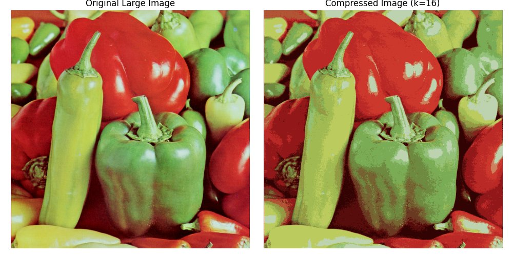
peppers-large.tiff file contains a 512x512 image of peppers represented in 24-bit color. To compress the image, we will cluster these points in color space into 16 clusters and replace each pixel with the closest cluster centroid.

❓5-a: K-Means Compression Implementation.

❓5-b: If we represent the image with these reduced (16 ) colors, by approximately what factor have we compressed the image?
📝 To represent 16 colors, we only need 4 bits, and one pixel of the original image needs 24 bits. The compression factor is: 24/4 = 6.

[Ke.dev @yangke687]

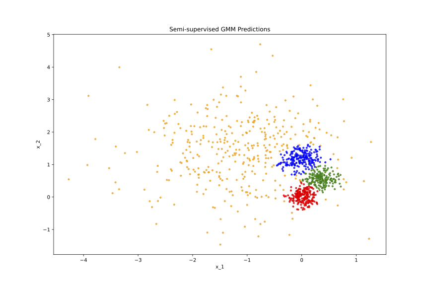
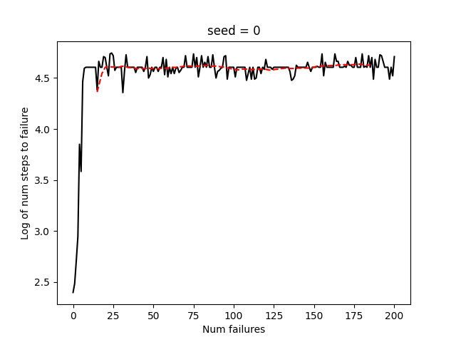
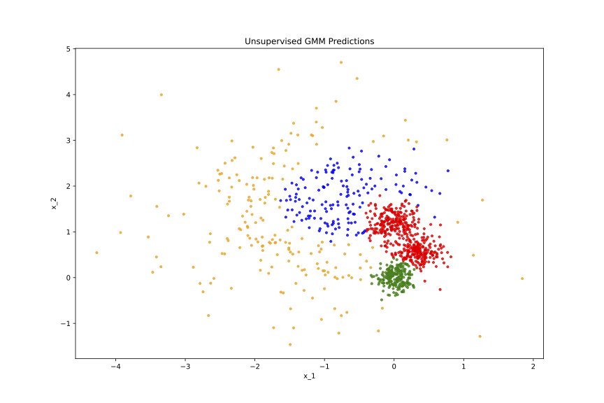
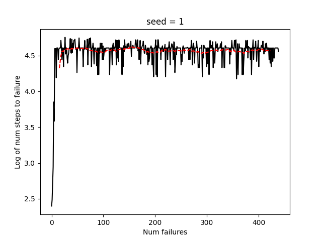
❓4-f: Comparison of Unsupervised and Semi-supervised EM.
i. Number of iterations taken to converge
ii. Stability
iii. Overall quality of assignments

📝i
Observation:
Semi-supervised EM generally takes fewer iterations to converge compared to unsupervised EM.

Explanation:
In unsupervised EM, the algorithm must explore a complex, multimodal log-likelihood landscape entirely from scratch, often taking many steps to shift and reorient the cluster parameters (especially for overlapping clusters). In semi-supervised EM, the labeled data points provide immediate and strong directional guidance for the cluster parameters (mu_j , sigma_j) from the very first iteration. This acts as an optimization shortcut, locking the components close to their true positions early on and accelerating overall convergence.

ii
Observation:
Semi-supervised EM exhibits significantly higher stability across different random initializations, whereas unsupervised EM is highly sensitive and unstable.

Explanation:
Unsupervised EM is notorious for getting trapped in sub-optimal local maxima or experiencing "label switching" depending on how the initial random groups are formed. If the initial partition is poor, a low-variance cluster might get swallowed by a high-variance one permanently. In contrast, semi-supervised EM introduces labeled anchors that permanently bind specific Gaussian components to their true corresponding semantic meanings. This strictly constricts the parameter space, ensuring that the algorithm consistently converges to the same global (or near-global) maximum regardless of random initialization.

iii
Observation:
The overall quality of assignments is substantially better in semi-supervised EM.

Explanation:
Unsupervised EM fails to recover this structure properly. Due to the lack of labels, the low-variance components expand or shift incorrectly to capture surrounding unlabelled points, causing severe overlap, distorted covariance shapes (like the stretched red cluster in the first plot), and misclassifying sparse background points into the wrong dense clusters.

Semi-supervised EM succeeds perfectly. The labels correctly isolate and anchor the three compact, low-variance clusters (red, green, and blue) into tight, high-density regions. Consequently, the fourth high-variance component (yellow) is properly identified as a broad, overlapping background cluster that correctly absorbs all the surrounding sparse data points.

[Ke.dev @yangke687]

CS229 (2018) problem set

In the standard unsupervised setting, we have m ∈ N unlabelled examples {x_1, ... x_m}. We wish to learn the parameters of p(x, z; θ) from the data. But z_i's are not observed. The classical EM algorithm is designed for this very purpose, where we maximize the intractable p(x; θ) indirectly by iteratively performing the E-Step and M-Step, each time maximizing a tractable lower bound of p(x; θ). Our objective can be concretely written as:

ℓ_unsup(θ) = ∑{i=1}^m log p(x⁽ⁱ⁾; θ)
= ∑{i=1}^m log ∑_{z⁽ⁱ⁾} p(x⁽ⁱ⁾, z⁽ⁱ⁾; θ)

Now, we will attempt to extend EM to the semi-supervised setting. Let us suppose we have an additional m~ ∈ N labelled examples {(x(1),z(1)),…,(x(m~),z(m~))} where both x and z are observed. We want to simultaneously maximize the marginal likelihood of the parameters using the unlabelled examples and the full likelihood of the parameters using the labelled examples by optimizing their weighted sum. More concretely, our semi-supervised objective can be written as:

ℓ_sup(θ) = ∑_{i=1}^m̃ log p( x̃⁽ⁱ⁾, z̃⁽ⁱ⁾ ; θ )
ℓ_semi-sup(θ) = ℓ_unsup(θ) + α ℓ_sup(θ)

We can derive the EM steps for the semi-supervised setting using the same approach and steps as before. You are strongly encouraged to show yourself (no need to include in the write-up) that we end up with:

E-step and M-step

❓4-a: First, we will show that this algorithm eventually converges. To prove this, it is sufficient to show that our semi-supervised objective ℓ_semi-sup(θ) monotonically increases with each iteration of the E and M steps. Specifically, let θ^(t) be the parameter obtained at the end of t EM-steps. Show that
ℓ_semi-sup(θ^(t+1)) ≥ ℓ_semi-sup(θ^(t))

📝We know
ℓ_unsup(θ) = ∑_{i=1}^m log ∑_{z⁽ⁱ⁾} Q_i(Z⁽ⁱ⁾) · [
P(x⁽ⁱ⁾, z⁽ⁱ⁾; θ) / Q_i(Z⁽ⁱ⁾) ]
1⃣
According to Jenson's inequation
log(E[x]) ≥ E[log(x)]

ℓ_unsup(θ) ≥ ∑_{i=1}^m ∑_{z⁽ⁱ⁾} Q_i(z⁽ⁱ⁾) · log[ P(x⁽ⁱ⁾, z⁽ⁱ⁾; θ) / Q_i(Z⁽ⁱ⁾) ]

Let L_unsup(Q, θ) = ∑_{i=1}^m ∑_{z⁽ⁱ⁾} Q_i(z⁽ⁱ⁾) · log[ P(x⁽ⁱ⁾, z⁽ⁱ⁾; θ) / Q_i(Z⁽ⁱ⁾) ]

We now have:
ℓ_unsup(θ) ≥ L_unsup(Q, θ);
L_unsup(Q, θ) is the lower bound of ℓ_unsup(θ)

L_semi-sup(Q, θ) = L_unsup(Q, θ) + α·ℓ_sup(θ)
L_semi-sup(Q, θ) is the lower bound of the objective

2⃣
In the E-step, setting Q_i(z⁽ⁱ⁾) = P(x⁽ⁱ⁾ | z⁽ⁱ⁾; θ) makes the lower bound tight at the current parameter θ^(t)
=> ℓ_unsup(θ^(t)) = L_unsup(Q^(t), θ^(t))
=> ℓ_semi-sup(θ^(t)) = L_semi-sup(Q^(t), θ^(t))

3⃣
In the M-step, θ^(t+1) is explicitly chosen to maximize
L_semi-sup(Q^(t), θ) with respect to θ:
👇
θ^(t+1) = arg max_θ L_semi-sup(Q^(t), θ)

Since θ^(t+1) maximizes this function, it must yield a value greater than or equal to the value at θ^(t).

L_semi-sup(Q^(t), θ^(t+1)) ≥ L_semi-sup(Q^(t), θ^(t))

4⃣
Finally, because L_semi-sup(Q^(t), θ^(t+1)) remains a valid lower bound for ℓ_semi-sup(θ^(t+1)) , we have:

ℓ_semi-sup(θ^(t+1)) ≥ L_semi-sup(Q^(t), θ^(t+1))

Chaining all the inequalities together gives:
ℓ_semi-sup(θ^(t+1)) ≥ L_semi-sup(Q^(t), θ^(t+1))
L_semi-sup(Q^(t), θ^(t+1)) ≥ L_semi-sup(Q^(t), θ^(t))
L_semi-sup(Q^(t), θ^(t)) = ℓ_semi-sup(θ^(t))

We have now proved:
ℓ_semi-sup(θ^(t+1)) ≥ ℓ_semi-sup(θ^(t))

❓4-b:
For Semi-supervised GMM E-Step. Clearly state which are all the latent variables need to be re-estimated in the E-step. Derive the E-step to re-estimate all the stated latent variables.

❓4-c:
For Semi-supervised GMM M-Step. Clearly state which are all the parameters need to be re-estimated in the M-step. Derive the M-step to re-estimate all the stated parameters. Specifically, derive closed-form expressions for the parameter update rules for
μ(t+1), Σ(t+1) and ϕ(t+1) based on the semi-supervised objective.

[Ke.dev @yangke687]

❓4-d: Classical Unsupervised EM Implementation.
📝run_em

❓4-e: Semi-supervised Em Implementation.
📝run_semi_supervised_em