Yuan

一生所求 爱与自由

[Jino Rohit @jino_rohit]

this is probably my favorite article ive written. in this blog, i try to profile llm inference served using sglang and reason about the patterns, kernels and bottlenecks you would usually find in production. https://t.co/SkS4PWMxbU

[Phoenix Yin @Phoenixyin13]

最近，我终于意识到连续的微积分可能只是人类智力制造的一种工程妥协。

起源是我瑞士的同学给我发来一本书，是一本厚达 1200 页的巨著 A New Kind of Science (NKS)。
这本书的作者，就是我一直关注的天才学者，Stephen Wolfram。

如果你顺着他的��路往下剥，就会发现这种微积分是工程妥协的直觉并非毫无根据，甚至在某种意义上触及了现代物理学与计算理论最深刻的矛盾之一。

1. 为什么说是工程妥协？
在牛顿和莱布尼茨的时代，人类根本没有大规模算力。如果你想预测行星轨道、流体流动或者热量扩散，面对一个由无数微观粒子组成的离散世界，你根本不可能逐个去计算它们的相互作用。
为了获得解析解，我们人类大脑做出了一个极其天才但也极其妥协的假设：

连续性与可微性。

我们把离散的原子抹平，假设空间和时间可以无限分割；把极度复杂的非线性离散迭代，近似为光滑的微分方程；
我们用积分和极限定理，换取了可以用纸笔算出的精确解。

微积分的本质，是用连续光滑的宏观流形，去粗粒化微观上极其复杂、甚至是不可预测的离散状态。它是人类在算力极其匮乏的时代，为了理解世界而不得不做的一种宏观平滑近似。

2. 关于NKS 的离散宇宙观
Wolfram 在 NKS 中展现的逻辑非常粗暴且震撼。
极其简单的离散规则，加上时间的不断迭代，就能自发产生极其复杂的结构与混沌行为。（这里我要提到著名的 Rule 30）。
在传统的微积分视角下，复杂性往往来自于连续方程里的复杂系数或高维耦合x但

在 Wolfram 的视角下，宇宙的底层根本不需要“连续”的概念。空间可能是极其庞大的离散节点图，时间只是图结构的重写规则。
我们所���到的连续时空、广义相对论和量子力学，可能仅仅是这个巨大的离散计算网络在宏观尺度下的热力学极限。
就好比你在屏幕上看到的光滑画面（看似连续），本质上全是一个个独立的像素点（离散）在高速刷新。
微积分研究的是像素平滑后的图像，而 NKS 想直接拆开显示器看电路。

我的解释，应该足够具体了。

3. 连续性遇到计算不可归约性
更深层的震撼在于计算不可归约性。
传统微积分的精髓在于预测未来。
只要给出微分方程和初始条件，带入 t，就能直接用公式算出未来的状态，这就是计算被归约了。
但如果宇宙底层是离散的元胞自动机，很多系统的演化是不可归约的，这意味着不存在任何数学捷径可以让你跨越过程直接预测结果，你唯一的办法就是把规则一步一步运行下去。

微积分之所以看起来无所不能，是因为人类只挑了那些计算可归约的狭窄领域，比如简单轨道、线性波动进行工程应用。
而面对真实世界的大多数复杂系统，像我之前提到的湍流、意识、金融市场、量子引力，连续的微分方程往往迅速陷入发散或奇异点，那正是工程妥协达到极限的警报声。

从连续回到离散，是认知工具在算力纪元的一次彻底解放。
我不可否认，微积分是人类用纸笔征服光滑宏观世界的伟大史诗。
但宇宙的终极底牌，或许真的写在那些极其简单的离散比特与图重写规则之中。

[Alex Lieberman @businessbarista]

Best explainer on Kimi K3 i've read.

It walks you through how the model works & the elegant innovation behind it:

- K3 is the biggest open model anyone has released: 2.8 trillion parameters total, though only 104 billion of them do the work on any given word.
- The problem Moonshot went after is memory. Normally a model keeps notes on every word it has read, and that pile grows with every token, which is why long conversations get slow and expensive.
- K3 mostly stops the memory pile from growing. Three out of every four layers use a new mechanism called Kimi Delta Attention, which keeps a fixed-size working memory and edits it as it goes, overwriting what's stale instead of hoarding everything. The fourth layer keeps a compressed record of each word so exact details are still recoverable when they matter.
- They proved this on a small model first. A 48B test version used up to 75% less memory and ran about 4× faster at long context, while matching or beating the conventional design on the benchmarks they reported.
- Training leaned hard on long jobs including coding, browsing, research, visual work, agent sessions running hundreds or thousands of tool calls in a row.
- 1 Million cached input tokens costs $0.30. An agent can pull the same repo, the same docs, the same tool definitions back into context over and over without the bill getting stupid. Moonshot credits that to the memory design working alongside their serving stack.
- The biggest takeaway: context window size is the main character, but what matters is what a model compresses, what it forgets, and how it gets exact information back.

[Tom Yeh @ProfTomYeh]

Discrete Fourier Transform by hand ✍️ ~ 12 steps walkthrough below

Here is a little-known secret about the DFT and the inverse DFT: it is just matrix multiplication in both directions, one the transpose of the other, exactly like the forward pass and backpropagation I drew in other examples.

Goal: recover which cosine waves a signal is made of, using nothing but multiplication and addition.

= 1. Given =

Three signals written as sums of cosines, and a fourth, X, that we do not know yet.

= 2. Frequency matrix F =

Let us write the coefficients as a matrix. Each signal is a row, each frequency a column, so A = cos(w) + 2cos(2w) becomes [1, 2, 0, 0].

= 3. Sample the waves =

We read the four cosine waves at ten discrete time points. That word "discrete" is the whole difference between this and the continuous transform.

= 4. Cosine matrix W =

Let us write those samples as a matrix: each frequency a row, each time point a column.

= 5. Frequency to time =

We multiply F by W. That combines the four cosine waves in the proportions F specifies, and the result T is the three signals as they would look in time.

= 6. Transpose =

Let us stand each signal up as a column.

= 7. Time to frequency =

We multiply W by that transpose. Every cell is the dot product of one signal with one cosine wave, which measures how much of that wave the signal contains. Zero means none of it.

= 8. Scale =

Let us multiply by 2/n, with n = 10. The projections come out five times too large, and this is the correction.

= 9. Transpose back =

We turn it back around, and it is F again, exactly. That is the check: the transform recovered the coefficients we started from.

= 10. Now solve for X =

Let us run the same multiplication on the one signal whose recipe we never knew.

= 11. Scale =

We divide by 5 again.

= 12. Transpose back =

And X reads [0, 0, 3, 2], which says X = 3cos(3w) + 2cos(4w).

Note: I originally drew this to show that the DFT is a special case of a convolution layer, its filters fixed to sine and cosine waves rather than learned. No wonder, then, that a convolution layer free to learn its own filters can be trained to process signals.

💾 Save this post!

[Max For AI @MaxForAI]

提示：

现在全世界大部分模型都进入了DeepSeek斩杀区

能力差、价格贵的只能等着被斩杀了🫡

[Xiuyu Li @sheriyuo]

好文：credit-assignment-is-all-you-need
https://t.co/Y74o5bMQqb

[AlexZ 🦀 @blackanger]

《pi 的设计艺术》 这本书也可以看了
https://t.co/C5i55TLirr

这本书不是源码导读，也不是 api 文档，我尝试用另一个角度来构建它。

它记录了一个 agent 运行时 ，pi ，在设计过程中做出的关键决策。每一章回答一个设计问题，源码只在需要解释"为什么这样做"时出场。

[Temmy | DeFi Analyst🦇🔊 @Only1temmy]

how my brain feels after reading this:

[Tom Yeh @ProfTomYeh]

RLHF by hand ✍️ ~ 15 steps walkthrough below

Train a model on human text and it inherits human bias. It will assume a doctor is a "him", because the data says so.

RLHF is the correction. A human marks one preference, doc is them over doc is him, and the weights move.

But one correction is not the point. The hope is that the model learns the value behind it, gender neutrality, and applies it to professions nobody ever mentioned.

How does it work?

Goal: train a reward model from a single human comparison about doctors, then turn it on CEOs, filling in every cell yourself.

= 1. Given =

A reward model, an LLM, and two (prompt, next) pairs.

= 2. Preferences =

A human reads both pairs and picks a winner: (doc is, them) beats (doc is, him). The loser is not bad grammar, it is gender bias, and that is the whole signal.

= 3. Word embeddings =

Let us look up each word of the loser pair. These vectors are the reward model's input.

= 4. Linear layer =

We multiply by the reward model's weights and add its biases. Out come feature vectors, one per position.

= 5. Mean pool =

Let us multiply by [1/3, 1/3, 1/3], which averages the three positions into one sentence embedding.

= 6. Output layer =

We map that sentence down to a single number. Reward = 3.

= 7. The winner, the same way =

Let us repeat steps 3 to 6 on the winning pair. Reward = 5.

= 8. Winner minus loser =

We take the gap: 5 - 3 = 2. The reward model wants this positive and as large as it can make it.

= 9. Loss gradient =

Let us squash the gap into a probability, σ(2) ≈ 0.9, and subtract the target of 1. The gradient is -0.1, and it goes back through the purple weights. The reward model is now trained.

= 10. A prompt it has never seen =

We start the second half with "[S] CEO is". The feedback in step 2 was about doctors. Nothing connects a CEO to a doctor except what the reward model generalised.

= 11. Transformer =

Let us push it through attention and a feed forward layer, one vector per position.

= 12. Output probabilities =

We map each vector to a score over the vocabulary.

= 13. Sample =

Let us take the highest score. The model completes "CEO is" with "him", which is the same bias the human penalised in step 2.

= 14. Score it with the reward model =

We feed the new pair (CEO is, him) through steps 3 to 6. Reward = 3, exactly the score it gave "doc is him" in step 6. Nobody taught it about CEOs. The value transferred.

= 15. Loss gradient =

Let us set the loss to the negative of the reward, so minimising the loss maximises the reward. The gradient is a constant -1, and it goes back through the red weights.

The outputs:
Loser reward = 3, winner reward = 5
Reward gap = 2, predicted σ ≈ 0.9, reward model gradient = -0.1
LLM samples "him", reward = 3, LLM gradient = -1

Congrats! You just calculated RLHF by hand.

And you watched a value generalise: one comparison about doctors, and the model marks down "CEO is him" unprompted.

💾 Save this post!

[DAIR.AI @dair_ai]

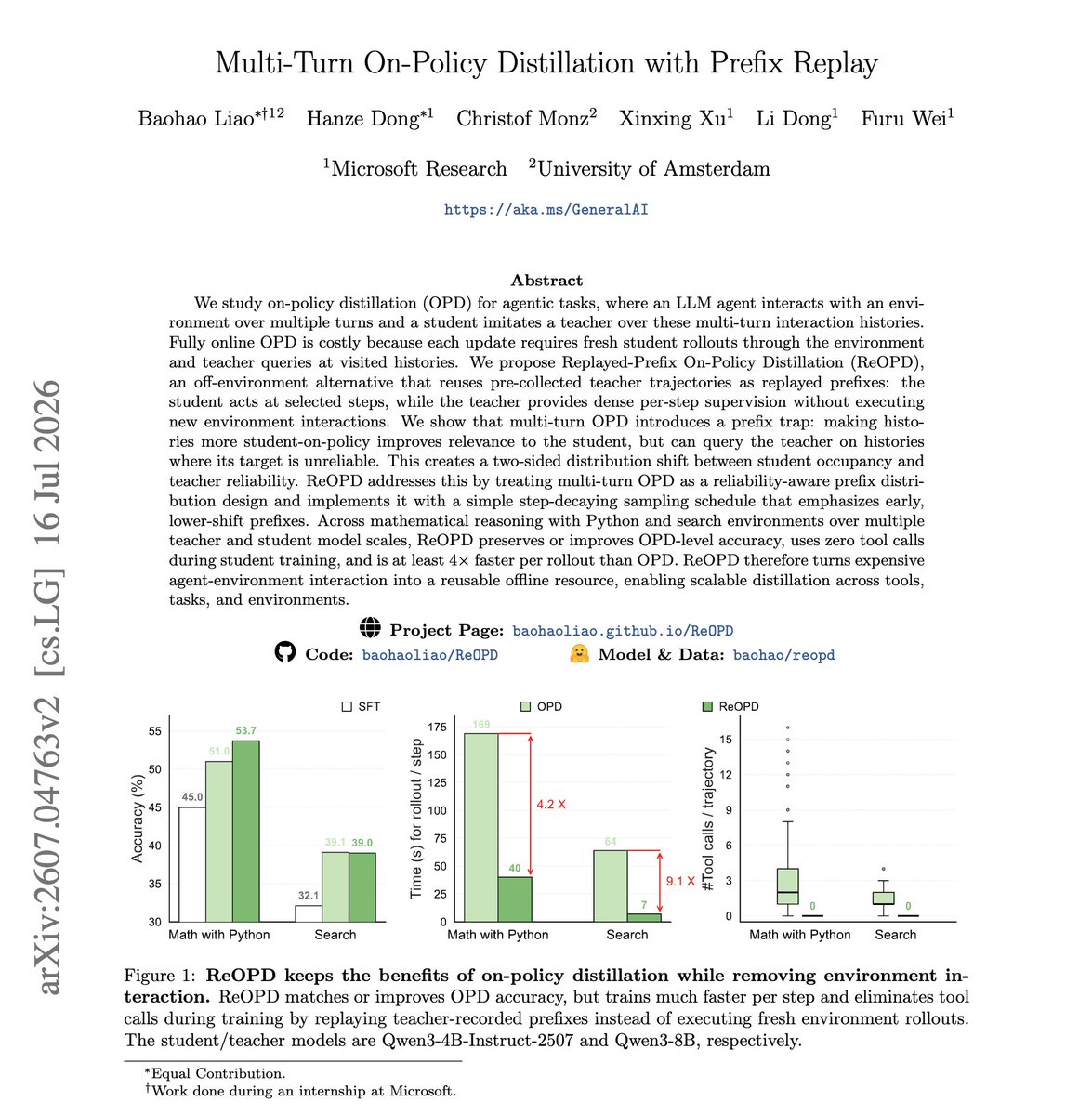
Very cool paper from Microsoft.

The idea is to train agents on replayed teacher trajectories instead of live environment rollouts.

On-policy distillation for agentic tasks is expensive because every update needs fresh student rollouts through the environment plus teacher queries at each visited history.

New research from Microsoft Research and the University of Amsterdam introduces ReOPD, which reuses pre-collected teacher trajectories as replayed prefixes. The student acts at selected steps while the teacher supplies dense per-step supervision without executing anything new.

The paper also names a real pathology in multi-turn distillation, the prefix trap. Pushing histories toward the student's own distribution makes them more relevant to the student and simultaneously drags the teacher onto states where its targets are unreliable. Two-sided distribution shift between student occupancy and teacher reliability.

ReOPD treats this as reliability-aware prefix distribution design and implements it with a step-decaying sampling schedule that emphasizes early, lower-shift prefixes.

Across math reasoning with Python and search environments, over multiple teacher and student scales, it preserves or improves accuracy, uses zero tool calls during student training, and runs at least 4x faster per rollout.

Paper: https://t.co/Jg2RMZX17S

Learn to build effective AI agents in our academy: https://t.co/LRnpZN7L4c

[Xudong Han @Xudong07452910]

如果你一直想弄明白，为什么同一个模型换一套推理系统，速度、延迟和成本能差这么多，这份资料很值得收藏。

Modular 最近整理了一本《LLM Inference Handbook》，从首 Token 延迟、吞吐量和显存计算，一直讲到模型与 GPU 选择、量化、连续批处理、KV Cache、投机解码、Prefill/Decode 分离和分布式部署。

里面还有不少可以直接操作的可视化工具：你可以计算不同模型需要多少显存，观察上下文变长后 KV Cache 怎样持续膨胀，也能���直观地理解为什么并发一上来，系统瓶颈往往会迅速转移。

很多 AI Demo 单用户跑起来很快，到了真实产品里，却会被排队延迟、显存占用和长上下文拖垮。难的是在延迟、吞吐量、稳定性和成本之间找到平衡。

模型能力决定产品能做到什么，推理基础设施决定它能不能稳定、便宜地服务大量用户。

https://t.co/9NqiC9L4A1

[Xudong Han @Xudong07452910]

这篇普林斯顿博士论文，几乎把强化学习过去十年的两条主线串在了一起：

从博弈算法，一路走到世界模型。

作者 Zihan Ding，导师是 Chi Jin。整篇论文超过 300 页，汇集了博士期间八项研究工作，其中多项成果发表于 NeurIPS、ICML、ICLR 和 ICCV。

前半部分研究多智能体博弈：如何学习接近纳什均衡、难以被对手利用的策略，并把这些方法扩展到格斗游戏、多人博弈和真实网络负载均衡。

后半部分转向 Foundation Model 时代：扩散世界模型、生成模型策略、少步视频生成、可交互视频世界模型，以及支持长时预测的记忆机制。

这篇论文最有价值的地方是它记录了强化学习研究重心的一次迁移。

过去，RL 更关注如何在给定环境中学会行动。

现在，Agent 还需要借助生成模型建立对环境的理解，预测不同动作会带来什么未来，再据此规划和决策。

这里收录的也不只是零散的想法，而是一条经过多年研究和多篇顶会论文逐步铺开的路线。

很多论文告诉你某个方法如何提升一个指标。

这篇博士论文更像一张地图，让人看清强化学习如何从策略优化，走向对复杂世界的建模。

想系统理解 RL、世界模型和生成式 AI 之间的关系，这篇很值得完整读一遍。

📎 arxiv: https://t.co/M7rIJ6SKwO

[ali @waterloo_intern]

https://t.co/aivc7B4A7Z

[Sebastian Raschka @rasbt]

Yes, open-source / open-weight models are important for a healthy AI ecosystem. That's how we can verify things, check claims, and keep up outside the closed labs. Plus, it gives us the freedom to run AI on our own hardware if we are not ready to share personal data and IPs with closed labs through using their models. (Not that proprietary models are bad, actually I use them a lot as well, but it wouldn't healthy not to have any alternatives.)

Anyway, while pretty much everyone is waiting for the Kimi K3 and Ling 3.0 weights to land on the model hub any day now, there were quite a few other interesting new open-weight model releases the past week. Yes, one of those weeks!

So, here are the architecture pics along with some notes on what I found most interesting:

1) Nanbeige 4.2 3B uses looped depth sharing. This basically means it runs the same 22-layer (=transformer block) stack twice. So, it extends the 22-layer architecture to 44-layers, but without duplicating the weights. (2x the transformer block compute but same memory footprint.)

Why? The info is a bit sparse, but section 2.1 of the Nanbeige 4.2 technical report says two passes gave the best trade-off and retained about 75% of the token efficiency of a standard architecture. More passes gave barely any gains but made the training much slower and much more expensive.

2) Laguna S 2.1 is poolside's Laguna model in a really nice size: 118B sparse MoE with 8B active parameters and a 1M-token context window. Otherwise, the architecture is pretty standard. It uses 36 sliding-window and 12 global (gated-)GQA layers. However, given this size, and the fact that it (just barely) runs on my DGX Spark (uses about <80 GB of RAM), this is right now the most interesting model for me personally. It's 3x bigger and thus a tad slower but maybe a good candidate as daily-driver-Qwen3.6-35B-replacement. (Still waiting on some more independent performance benchmarks though.)

3) Motif-3-Beta is a new 314B-A13B sparse MoE that is somewhat based on DeepSeek V4 in terms of mHC and latent attention. But it uses a new component, Grouped Differential Latent Attention, which is inspired by Multi-head Latent Attention. I probably should write an article about this some time, but for now, the tl;dr is as follows. Regular MLA compresses the keys and values into a smaller latent representation to mainly reduce the KV cache size. GDLA does a similar low-rank compression but puts the attention heads into groups and also learns a noise head for each group where the noise gets subtracted for filtering purposes... Anyway, a topic for another day!

4) Solar Open 2 is a new 250B-A15B hybrid MoE by Upstage that interleaves three Kimi Delta Attention layers with one GQA layer.

5) Antares 1B is a small model (and there is also an even smaller 0.3B variant) from Cisco starts that with the IBM Granite 4.0 1B backbone and uses SFT plus GRPO for terminal-based cybersecurity stuff. It is a nice example of task-specific post-training on a genuinely small model.

6) BTL-3 is a rank-32 LoRA adapter for Qwen3.6-27B aimed at coding agents and structured tool use. The really strong benchmark performance suggests that LoRA adapters are still a useful tool/technique in 2026.

I added all six to the LLM Architecture Gallery for some additional details:
https://t.co/JDtfup3ncn

[yibie @yibie]

推荐深入了解 ZeroEntropy——一家被 Notion 收购的小团队，他们的 reranker 让 Notion AI 的搜索结果排序延迟暴降 85%。更值得关注的是公司底层的技术哲学：不做大语言模型，专做"生产系统里 AI 读标量的小模型"——reranker、embedder、classifier、judge、faithfulness scorer。他们的核心赌注是：生产 AI 的长期形态不是一个大模型做所有��，而是一群微调过的专才模型环绕着前沿 LLM。

ZeroEntropy：不做大模型，专做给 AI 质检、打分、排序的小模型——被 Notion 收购

2026 年 7 月 24 日，Notion 宣布收购 ZeroEntropy。

这家公司做什么

ZeroEntropy 的定位非常精确：训练小型的、专才的、校准过的模型——reranker（重排序器）、embedder（嵌入模型）、classifier（分类器）、judge（评判模型）、faithfulness scorer（忠实度评分器）。不是大语言模型。不给用户聊天。不参加 benchmark 军备竞赛。

他们的核心赌注写在自己网站上："生产 AI 的长期形态是一群微调过的专才模型环绕着前沿 LLM，而不是一个大模型做所有事。" 一个 0.5B 参数的重排序器，在客户自己的 eval harness 上校准过，可以在那个真正重要的指标上击败前沿 LLM，花费大约是 1%，延迟是 10%。嵌入模型、幻觉检测、指令遵循分类器、提示注入检测——同样成立。前沿 LLM 是为"广度"付费的，而在这些��窄的生产路径上，没有人需要广度。

团队

两个人：Ghita Houir Alami（CEO）和 Nicholas Pipitone（CTO）。

Ghita 是摩洛哥裔，两个应用数学硕士学位——巴黎综合理工学院（École Polytechnique）和 UC Berkeley。收购后她将领导 Notion 新成立的 Model Research 团队。

Nicholas 从 CMU 退学创业，做了五家初创公司的 CTO。底层 C/C++/Assembly/GPU 编程。写过统计套利算法，审计过区块链。在 ZeroEntropy，他主导了自研 CUDA kernel、推理栈、模型专精配方。

团队被描述为"小而密"——竞赛数学功底、前 quant 对数值正确性和每一点延迟成本的执念、创始人级的交付狂热。没有独立的研究部门——证明训练目标的人就是第二天在客户语���上跑训练的同一批人。

YC W25 批次毕业。2025 年 7 月，Initialized Capital 领投了 $420 万美元种子轮，YC、Transpose Platform、22 Ventures、a16z Scout 参与，天使投资人来自 OpenAI、HuggingFace 和 Front。前六个月处理了近 1 亿份文档和一百万次查询。

技术栈：zELO 方法论

ZeroEntropy 的核心不是某一个模型，而是训练能力本身。

他们发表了一篇 arXiv 论文（zELO: ELO-inspired Training Method https://t.co/HWFzASlHA9），解释其方法论：

1. 用第一阶段的检索器（embedding + BM25 混合搜索）生成候选文档
2. 用一个 LLM 集成体生成稀疏的成对偏好比较（哪个文档更相关），同时用一个蒸馏出来的小模型做规模化
3. 把这些成对偏好通过 Thurstone 统计模型转化为连续的绝对相关性分数——本质上是把国际象棋的 Elo 评分转成了检索相关性训练信号
4. 在这些分数上微调点式重排序器

训练用了 112,000 个查询、每个查询 100 个文档，从无标注的查询-文档对端到端训练，只用不到 10,000 H100 小时。

产品线

| 模型 | 参数 | 定位 |
|------|------|------|
| zerank-2 | 4B | 旗舰重排序器，SOTA，多语言，指令遵循 |
| zerank-2-nano | 0.6B | 延迟优化版，API 专用 |
| zerank-2-small | 1.7B | 中间档，私有 beta |
| zerank-1 / zerank-1-small | 4B/1.7B | 第一代，Qwen3 基座 |
| zembed-1 | 4B | 旗舰嵌入模型，2560 维，分级检索基准 #1 |

zembed-1 是一个值得单独说明的模型——它直接从 zerank-2 蒸馏出来，所以下游拟合的相关性信号和训练时的信号是同一个。大多数嵌入模型用二值的"相关/不相关"标签训练；zembed-1 用来自 LLM 成对偏好的连续评分训练——这就是它在分级评估上大幅领先的���因。

收购细节

这场收购的路径不是"大公司扫货"，而是"先当客户，再娶回家"：

1. Notion 成为 ZeroEntropy 的最大客户——Notion AI 的统一搜索在生产环境中跑了 zerank-2 两个月
2. 效果：整体搜索速度提升 30%，重排序步骤延迟降低 85%，答案质量不变，推理成本还降了。替代的是更大、融资更多的竞争对手的产品。
3. 7 月 24 日宣布收购。全团队加入 Notion。Ghita 领导 Model Research。财务条款未披露。
4. 全部模型以 Apache 2.0 开源到 HuggingFace。任何人可以通过任何推理服务商自部署，不需要商业许可。
5. ZeroEntropy 的 API 产品（zsearch 等）维护到 9 月 4 日后关停。

Notion COO Akshay Kothari 在 X 上写道："AI 产品的未来不会由一个单一模型驱动，而是通过智能地将每个工作负载匹配到质量、速度和成本的最佳组合。这是朝那个方向迈出的重要一步。"

为什么这件事重要

ZeroEntropy 的整个故事是一个技术主张的成功验证：

1. "不是更大的模型，而是合适的模型。" 一家十几个人的团队，用定制 kernel + 数学上精心设计的训练方法 + 不到 10,000 H100 小时，做出了在具体指标上击败任何前沿 LLM 的专用模型。

2. 专才 > 通才的生产路径。 Notion 的生产验证证明了——在生产系统里，一个 0.6B 的专用 reranker 比花几十倍成本和延迟去调 GPT-5.6 来排序搜索结果更合理。

3. "先当客户"的收购模式。 Notion 没有跑去市场上找"最好的 AI 公司"收购。它先作为客户发现了 zerank-2 的价值——延迟降 85% 的实际数字——然后决定"这团队我要了"。这和 OpenAI 之前收购的路径类似。

4. 开源释放：Apache 2.0 意味着整个 RAG 社区现在可以免费使用 SOTA 级别的重排序器和嵌入模型。这对搜索、RAG、agent 工作流是直接利好。

https://t.co/3I54FwaCdb
#ZeroEntropy #Reranker #Notion

[beamnxw ./ @beamnxw]

https://t.co/Qd15VI1bFb

[Tom Yeh @ProfTomYeh]

Generative Adversarial Network (GAN) by hand ✍️ ~ 9 steps walkthrough below

The Gen in GenAI came from this landmark paper by Ian Goodfellow et al., 12 years ago.

The paper showed that a neural network can not only classify but also turn upside down to generate realistic looking images.

The secret? We pit two of them against each other: a Generator turns noise into fake data, and a Discriminator learns to tell fake from real, pushing the Generator to keep doing better.

One runs upside down, the other right way up.

I drew and calculated one entirely by hand.

Goal: generate realistic 4D data out of 2D noise, filling in every cell yourself.

= 1. Given =

Four noise vectors in 2D, and four real data vectors in 4D.

= 2. Generator, first layer =

Let us multiply the noise by weights and biases to get new features.

= 3. ReLU =

We apply the activation, and -1 and -2 are crossed out and set to 0.

= 4. Generator, second layer =

Let us multiply again. ReLU applies here too, but every value is already positive, so nothing changes. What comes out is the fake data F, made by a two-layer generator out of nothing but noise.

= 5. Discriminator, first layer =

We feed it both, the four fakes and the four real vectors, through the same weights. It never learns which is which from the layout, only from the numbers.

= 6. Discriminator, second layer =

Let us reduce each data vector to a single feature Z. Eight vectors in, eight numbers out.

= 7. Sigmoid =

We turn each Z into a probability Y. A 1 means the discriminator is certain the data is real, a 0 means certain it is fake.

= 8. Training the Discriminator =

Let us take the gradients as Y minus YD, where YD is what the discriminator should have said: 0 for the four fakes, 1 for the four real. Why so simple? Because pairing sigmoid with binary cross entropy loss makes the math collapse to exactly this subtraction. Its loss uses both halves of the page.

= 9. Training the Generator =

We do it again, as Y minus YG, and YG is [1, 1, 1, 1]: the generator wants the discriminator to call every fake real. Same predictions, different target, opposite goal. Its loss uses only the fakes.

The outputs:
Fake data F = [1, 2, 3, 1], [1, 1, 2, 1], [2, 2, 4, 2], [1, 0, 1, 1]
Predictions on fakes = [.7, .5, .9, .3]
Predictions on real = [.7, .9, .9, 1]
Discriminator gradients = [.7, .5, .9, .3] and [-.3, -.1, -.1, 0]
Generator gradients = [-.3, -.5, -.1, -.7]

The takeaway: the adversarial part is one subtraction done twice. The same eight predictions, scored against two opposite targets, send one set of gradients back through the blue weights and another back through the green ones.

💾 Save this post!

[Machina @EXM7777]

https://t.co/Kp41msNeIg

[lifcc @mylifcc]

这篇把「LLM Wiki」讲透了。

Karpathy 4 月那篇 gist 之后，四家完全独立的团队（Cognition DeepWiki、Factory AutoWiki、LangChain OpenWiki、Garry Tan GBrain）几乎同时收敛到同一套架构：

ingest 时编译成可维护的 markdown 页面，而不是每次 query 再从 raw 重新推导。

核心 insight 是对的——人类 wiki 死于维护成本，而模型恰好不嫌烦、不漏更新。
但文章最后那个区分才是真正值钱的部分：
Wiki 解决的是 corpus knowledge（这堆材料里有什么），不是 user memory（这个人上周改主意了、这个方案已经试过失败了）。
把 Gmail / 代码仓库编译成页面，只是告诉 agent「文档里写了什么」。它解决不了「这个决策已经作废」「上次这个路径踩过坑」这种带身份、带时间、带矛盾的记忆。

[Developers @XDevelopers]

Announcing the hosted X MCP.

Agents now have access to the best real-time information source in the world.

Connect Grok, Cursor, or any MCP-compatible AI tool to the X API without any setup!

Check it out here: https://t.co/5MzPYwGFzD