Andrés A León

Hincha de Millonarios FC ║ Ingeniero Electrónico

[VSports Team @VSportsTM]

La MLS tuvo su Valderrama Day. Así como leen. Fue en 1996. Coincidió con Tampa Bay Mutiny-Kansas City Wizards. Se sumaron hasta los encargados de las transmisiones. Hoy el colombiano cumple 65 años 🇨🇴❤️

[CHAVERRA BALÓN DE ORO 2027 @pafoira]

#ESPNF90Colombia

-Marocco: no tenia sostén Bustos
-@udsnoexisten, Sarah Castro y Marocco: 😂😂😂

[Matheorems @matheorems]

An infinite bell curve hides a circle.

The volume under z = e^{-(x² + y²)} across the entire plane equals π.

In polar coordinates the integral separates:
∫₀^{2π} ∫₀^∞ e^{-r²} r dr dθ = 2π · ½ = π
This identity underpins the normal distribution, the heat equation, quantum ground states, and the Gaussians that shape modern machine learning.

Infinity can be finite when symmetry is complete.

[Philosophy Of Physics @PhilosophyOfPhy]

Visualization of How an Electromagnetic Wave Travels.

[ElectronicsNotes by Ian Poole @ElecNotes]

Logic Truth Tables - a back to basics guide

Getting back to basics is sometimes the best way to master complex digital systems.

Whether you are designing a simple circuit or working on advanced embedded systems, understanding Logic Truth Tables is the essential foundation.

These tables define exactly how logic gates process binary information, forming the building blocks of all modern electronics.

I’ve put together a comprehensive infographic that summarizes the core logic functions you need to know:

✅ Buffer & Inverter (NOT)
✅ AND & NAND
✅ OR & NOR
✅ Exclusive OR (XOR) & Exclusive NOR (XNOR)

This guide includes the symbols, Boolean operations, and truth tables all in one place to help streamline your design process.

📌 Check out the full infographic linking the comments.

What’s your "go-to" logic gate when solving a tricky design problem? Let’s discuss in the comments! 👇

#Electronics #DigitalLogic #Engineering #circuitdesign #truthtable #digitaldesign #STEM #electronicsnotes

[The Math Mastery @naturevx0]

“Master These 9 Summation Formulas and Make Maths Easier!”

[RayPCB @RaymingTech]

DC/DC Topologies Overview (Part 2): Isolated Converters 📍

DC/DC topologies are everywhere—from consumer gadgets to industrial control systems.
Here, I’ll focus on industrial control as a practical reference.

🔌 When do we need isolation?
• Safety compliance
• Noise separation
• High-voltage domains
• Field wiring protection

Let’s break down the most common isolated topologies 👇

🟡 Flyback
The go-to for low-to-mid power.
✔ Simple & cost-effective
✔ Easy multi-output
Widely used in PLC power modules and sensor interfaces.

🟡 Forward
Better efficiency than Flyback.
Ideal for medium-power industrial supplies where efficiency matters.

🟡 Push-Pull / Half-Bridge
When power levels rise.
Found in motor control drives and distributed power modules.
⚠️ Transformer balance and layout symmetry are critical here.

🟡 Full-Bridge
Built for high-power systems.
Typical in industrial UPS and large power cabinets.

🟡 LLC Resonant
Modern, high-efficiency solution.
✔ Soft switching (ZVS)
✔ Lower EMI
✔ Higher efficiency
Regulated via switching frequency (not duty cycle).
Common in high-performance power supplies.

🔎 Industrial Design Insight
In isolated power design, you must balance:
• Power level
• Isolation class
• EMI compliance
• Thermal management
• Manufacturability

Transformer layout, creepage distance, and grounding strategy often separate success from failure.

💡 Good power design must pass safety, EMI, thermal, and production consistency—not just simulation.

What’s your go-to topology for isolated designs? Let’s discuss in the comments 👇

#PowerElectronics #DCDCConverter #IsolatedConverters #IndustrialControl #HardwareDesign

[RayPCB @RaymingTech]

In 1964, operational amplifiers were already being treated as far more than simple amplifiers. This application chart, published by George A. Philbrick Researches, Inc. in August 1964, was titled: “Typical Operational Amplifier Applications for Modelling, Measuring, Manipulating & Much Else” The page presents 25 classic op-amp applications, including voltage sources, bridge amplifiers, charge amplifiers, current-to-voltage converters, integrators, differentiators, precision rectifiers, AC-to-DC converters, logarithmic amplifiers, oscillators, PID controllers, negative-impedance circuits, and impedance converters. What impressed me most was not the complexity of any single circuit. It was the underlying design philosophy. The operational amplifier was being used as a general-purpose analog computing and signal-processing building block. Its input could represent voltage, current, charge, impedance variation, or bridge imbalance. Its output could perform amplification, integration, differentiation, rectification, comparison, oscillation, or even synthesize a negative impedance. Many circuit structures that still appear in analog electronics courses, design textbooks, and sensor readout systems were already remarkably mature in this 1964 document. This is why I chose this figure as the first entry in my circuit-analysis series. It is a useful reminder that learning operational amplifiers is not merely about understanding a triangular symbol or memorizing a collection of standard circuits. It is about learning a language for manipulating analog signals.

[SparkED @Afghan_Engineer]

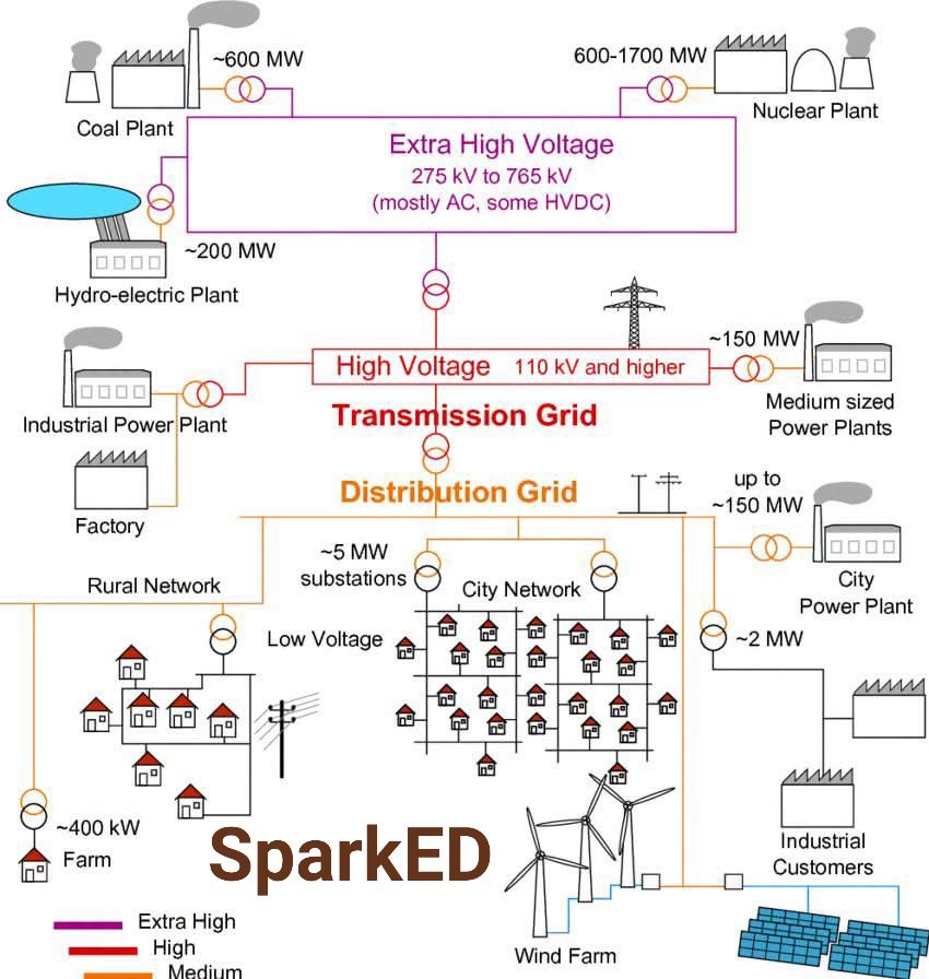
SYNCHRONOUS vs ASYNCHRONOUS POWER SYSTEMS — WHAT’S THE DIFFERENCE?

Ever wondered what makes two power grids operate together or prevents them from being directly connected?

🔹 Synchronous System:
Two or more grids operate at the same frequency and remain phase-synchronized, allowing AC power to flow directly between them.

🔹 Asynchronous System:
The grids operate at different frequencies or are not phase-synchronized. They cannot be directly interconnected with a normal AC tie.

How can asynchronous grids exchange power?
Through HVDC links or frequency converter stations, which act as an interface between the two systems.

🇯🇵 Example: Japan has 50 Hz and 60 Hz regions, connected through frequency-conversion facilities.

In simple terms:
Synchronous = same frequency + synchronized phase.
Asynchronous = not synchronized, requiring an interface to exchange power.

This is where power electronics meets power systems.

[The Scientific Lens @LensScientific]

The Gaussian integral appears throughout probability and statistical physics.

The Lorentzian describes resonance and spectral line shapes.

The sinc integral is central to Fourier analysis and the mathematics of reconstructing signals from discrete samples.

[Millonarios FC Femenino @MillosFcFem]

+1000 DE AURA Ⓜ️✨

[RayPCB @RaymingTech]

Ever wondered how two devices talk to each other without a shared clock?
That’s where UART (Universal Asynchronous Receiver/Transmitter) comes in.

UART is a simple, reliable serial communication protocol widely used in embedded systems. No clock line needed — just two wires and a matching speed.

🔧 Key Features
✅ Asynchronous – no clock signal
✅ Full‑duplex – send & receive simultaneously
✅ Only 2 lines: TX (transmit) and RX (receive)
✅ Predefined baud rate required (e.g., 9600, 115200)

⚙️ How it works (frame format)
➡️ Start bit (LOW)
➡️ Data bits (5–9 bits, LSB first)
➡️ Parity bit (optional – error detection)
➡️ Stop bit(s) (HIGH)

🔄 Basic flow

Microcontroller sends parallel data

UART converts to serial

Bits transmitted one by one via TX

Receiver UART reads via RX

Serial converted back to parallel

Data delivered to receiving device

📊 Example
Transmitting 0xA5 (10100101) at 9600 baud:
Start → 1 0 1 0 0 1 0 1 → Stop

📍 Real‑world applications

MCU ↔ PC communication

GPS modules

Bluetooth modules (HC‑05, HC‑06)

Serial debugging

⚠️ Critical note
Both sides must use the same baud rate — otherwise, no communication.

💡 Why UART matters
It’s simple, cost‑effective, and still the backbone of embedded communication.

👉 Found this useful? Repost to help others debug their serial connections.
♻️ Follow me for more embedded systems & electronics insights.

[Cosmos Archive @cosmosarcive]

Electricity and magnetism are not separate stories. They are two sides of the same field.

In 1820, Hans Christian Ørsted noticed that a current carrying wire could deflect a compass needle, revealing that electric current produces a magnetic field. Faraday later showed the reverse: changing magnetic fields can induce electric fields.

The key equations are:

∇ × E = −∂B/∂t
∇ × B = μ₀J + μ₀ε₀ ∂E/∂t

That connection is the foundation of electromagnetism, from generators to electromagnetic waves.

[PY6CJ - João Grisi @py6cj]

Understanding the Nyquist-Shannon Sampling Theorem is fundamental in modern amateur radio, especially when operating transceivers and receivers based on SDR (Software Defined Radio).

Read the full text at:
https://t.co/MsmgAziB8L

Vídeo of: https://t.co/9FJseMX2Br

Text : PY6CJ

[The Scientific Lens @LensScientific]

Bernoulli’s principle connects pressure, velocity, and energy in a flowing fluid.

Where the flow speed increases, the static pressure decreases, and where the flow slows down, the static pressure increases, provided the conditions for Bernoulli’s equation are satisfied. This pressure difference is one of the key pieces in understanding how aerodynamic lift is produced by wings. The same principle also appears throughout fluid dynamics, from aircraft and birds to flowing water and ventilation systems.

[SparkED @Afghan_Engineer]

Salt & charcoal have traditionally been used to help improve soil conductivity.

Salt increases the electrolyte content, while charcoal helps retain moisture.

But, they can accelerate electrode corrosion & contaminate soil, so modern earthing systems use earth enhancement materials instead.

[RayPCB @RaymingTech]

From 0.2V to 3.6V: What a Motor Current Sensing Amplifier Really Does

In motor control, the current signal is often far smaller than most people expect.

A low-value shunt resistor might generate only a few hundred millivolts — yet that tiny voltage is exactly what the control system relies on to understand the motor’s behavior.

So the real challenge isn’t just sensing current.
It’s turning a very small, noise-sensitive signal into something the MCU can read accurately.

🟠 The original signal is small, but the environment is noisy
In a BLDC drive, phase current is typically measured through a low-value shunt resistor.
Example: with a 20 mΩ shunt, even 10 A of current produces only 0.2V differential.
That signal exists inside a switching environment full of MOSFET noise, ground disturbances, and EMI.

🟠 The amplifier does more than just increase voltage
A differential amplifier stage is commonly used here.
Its job: amplify the shunt voltage while rejecting common-mode disturbance.
In practice, it does two things at once:
• Makes the signal larger
• Makes it more usable

🟠 Gain and offset make the signal ADC-friendly
With only 0.2V at the input, ADC resolution and electrical noise become major issues.
After amplification, the signal can reach 1.2V, 2.4V, or even close to 3.6V — depending on gain and system requirements.

Many real designs also shift the output upward by a reference voltage (since ADCs typically can’t accept negative inputs).
Instead of 0 A = 0V, designers create a new center point, e.g.:
• 0 A = 1.25V
Then:
• Positive current → output above 1.25V
• Negative current → output below 1.25V

That’s the real meaning behind “from 0.2V to 3.6V”: a tiny shunt signal is translated into a voltage range the MCU can actually read.

🟠 A correct schematic can still give poor measurements
Even when the circuit looks right, current sensing can fail due to:
• Shunt resistor temperature drift
• Resistor ratio accuracy
• Unstable reference voltage
• Noisy routing
• Poor grounding and return path control

When the measured voltage is this small, layout and implementation matter just as much as the calculation.

📌 Takeaway
A motor current sensing circuit is a great reminder that analog design is often about translation.
A tiny voltage must be amplified, shifted, and protected from noise before it becomes useful control data.

[academi study w @academiastudygd]

C++ · Physics · Calculus — Integrated Stem Bundle for CS students https://t.co/UB1za8qrob

[The Math Flow @TheMathFlow]

Johann Bernoulli posed the problem to the mathematicians of Europe in 1696; it remains vital today in quantum mechanics and many other fields.

If a ball is to roll down a ramp which connects two points, what must be the shape of the ramp's curve, such that the descent time is a minimum?
Intuition says that it should be a straight line. That would minimise the distance, but the minimum time happens when the ramp curve is a cycloid.