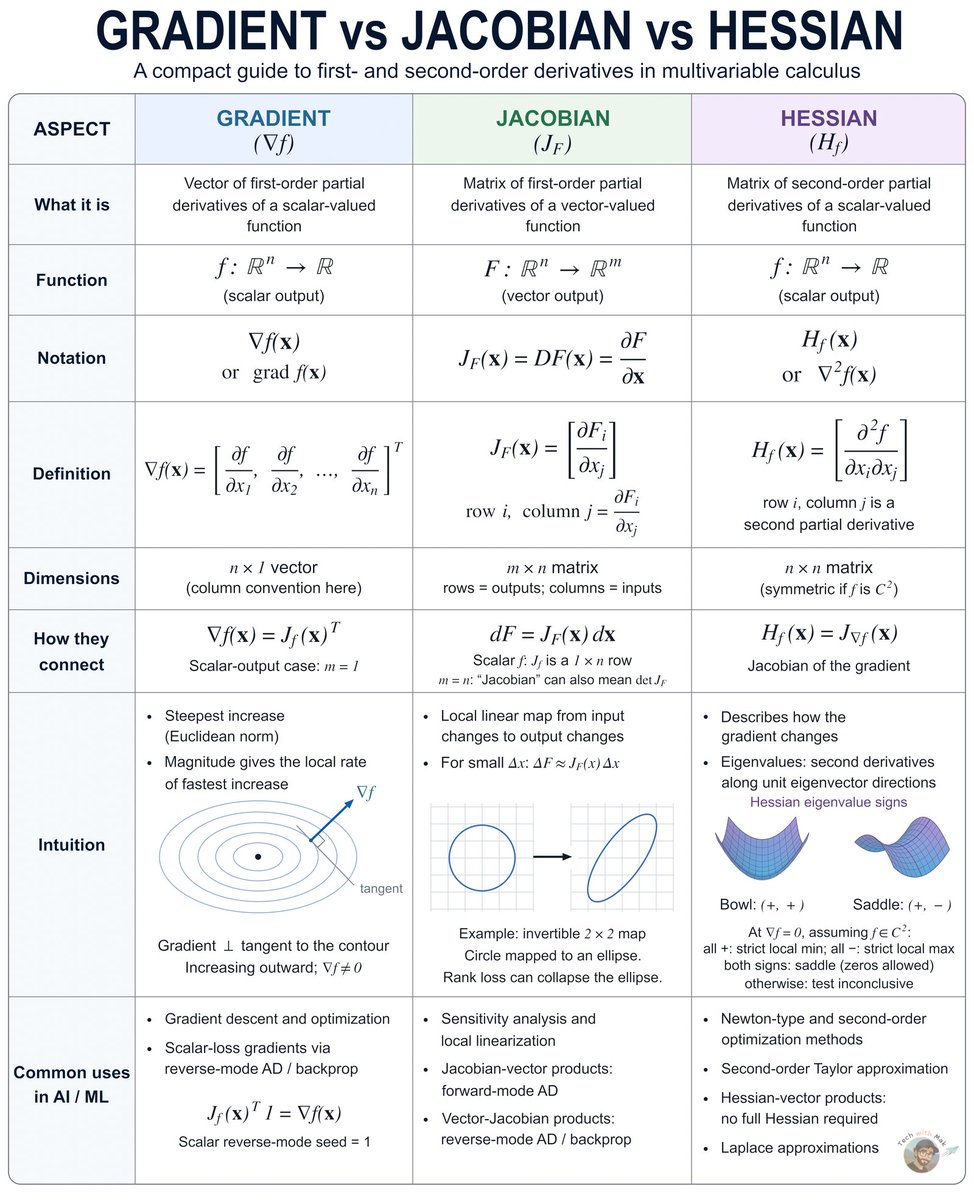
This math sits underneath nearly every AI model being trained right now.
Gradient. Jacobian. Hessian.
Three words that look intimidating at first. But they are really just three ways of measuring change.
(Throughout, assume the functions are smooth enough to differentiate.)
𝟭./ 𝗚𝗿𝗮𝗱𝗶𝗲𝗻𝘁 ∇f
Takes a scalar function:
f : ℝⁿ → ℝ
Returns a vector of n first-order partial derivatives (written as a column here).
It answers:
"Which direction makes f increase fastest?"
That is why gradients are central to optimization.
Gradient descent steps in the opposite direction, because the gradient points uphill.
Backpropagation is how we compute gradients efficiently during training.
𝟮./ 𝗝𝗮𝗰𝗼𝗯𝗶𝗮𝗻 J_F
Takes a vector-valued function:
F : ℝⁿ → ℝᵐ
Returns an m × n matrix of first-order partial derivatives.
It answers:
"How does each output change with each input?"
The Jacobian is the local linear map of F:
ΔF ≈ J_F(x) Δx for small Δx
It shows up in:
→ sensitivity analysis and local linearization
→ change of variables (through its determinant, when m = n)
→ automatic differentiation:
• forward-mode AD computes Jacobian-vector products
• reverse-mode AD (backprop) computes vector-Jacobian products
When m = 1, the Jacobian is just the gradient written as a row.
𝟯./ 𝗛𝗲𝘀𝘀𝗶𝗮𝗻 H_f
Takes a scalar function:
f : ℝⁿ → ℝ
Returns an n × n matrix of second-order partial derivatives.
It answers:
"How does the gradient itself change?"
That is why the Hessian captures the local curvature of f.
When the second partial derivatives are continuous, the Hessian is symmetric.
At a critical point (where ∇f = 0):
→ positive definite Hessian → strict local minimum
→ negative definite Hessian → strict local maximum
→ indefinite Hessian → saddle point
→ semidefinite Hessian → inconclusive
It powers Newton-type and other second-order optimization methods, and uncertainty approximations such as the Laplace approximation.
𝗧𝗵𝗲 𝗰𝗹𝗲𝗮𝗻 𝗺𝗲𝗻𝘁𝗮𝗹 𝗺𝗼𝗱𝗲𝗹
Gradient = first derivatives of one output
→ tells you direction
Jacobian = first derivatives of many outputs
→ tells you sensitivity
Hessian = second derivatives of one output
→ tells you curvature
And they connect:
∇f = (J_f)ᵀ for scalar f (row vs. column convention)
H_f = the Jacobian of ∇f
Same idea:
measure change.
Different object:
direction, sensitivity, curvature.
Once this clicks, optimization stops looking like a pile of formulas.
It starts looking like a map of the problem.
Navier–Stokes and OpenAI’s New Advance
The Navier–Stokes equations describe the motion of viscous fluids:
∂ₜu + (u·∇)u = −∇p + νΔu, ∇·u = 0.
The famous Navier–Stokes existence and smoothness problem asks whether every smooth initial condition in 3D remains smooth for all time, or whether a finite-time singularity can develop.
OpenAI has now announced an AI-generated proof claiming that smooth solutions can indeed develop a singularity in finite time. Its system reportedly used around 10,000 AI agents working in parallel, with the resulting argument formally checked in Lean.
An important part of the mathematical story, however, predates this announcement. The blow-up programme of Diego Córdoba and Luis Martínez-Zoroa, including their work with Fan Zheng, established crucial finite-time blow-up results for related forced/hypodissipative Navier–Stokes models.
Thus, the recent development should be viewed in the context of this broader mathematical programme: Córdoba and Martínez-Zoroa developed key ideas underlying the route toward blow-up, while OpenAI claims to have pushed such ideas to the classical 3D Navier–Stokes problem.
If independently verified, this would be a historic advance—not only for fluid dynamics, but also for AI-assisted mathematical discovery.
Diego Córdoba and Luis Martínez-Zoroa, whose foundational blow-up programme is an important precursor to this line of work.