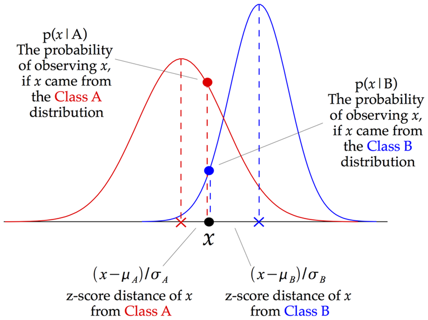
Gaussian Naive Bayes is a simple yet powerful probabilistic classifier based on Bayes' theorem. It "naively" assumes that all predictive features are independent of one another. The "Gaussian" variant is tailored for continuous data, operating under the assumption that the features for each class follow a normal (Gaussian) distribution. This simplicity makes it incredibly fast and effective, establishing it as a strong baseline model in machine learning, especially for high-dimensional datasets. Real-world applications are widespread: it's used in text classification, medical diagnosis (e.g., predicting diseases from lab results), and classic email spam filtering.
Image source: https://t.co/0ouJPRkrB9
Missing data is a common issue in data analysis, and there are several approaches to handle it depending on the data structure and analysis requirements. Each method has its advantages and limitations, and choosing the right one is crucial for ensuring the accuracy and robustness of your results. Below, you can find some popular methods to handle missing data.
1️⃣ Listwise Deletion
This method removes rows with missing values entirely. While it simplifies analysis, it can lead to a significant loss of data, reducing sample size and statistical power. If the data is not missing completely at random (MCAR), listwise deletion is likely to introduce bias into the analysis, potentially distorting results.
2️⃣ Single Imputation
Single imputation methods, such as regression imputation or predictive mean matching, replace missing values with a single plausible estimate. These methods are straightforward to apply but do not account for the uncertainty associated with missing values.
3️⃣ Multiple Imputation
Multiple imputation addresses the limitations of single imputation by creating several plausible imputed data sets. The results from these data sets are then combined, providing a more robust approach that accounts for the variability introduced by missing data.
The attached image illustrates the structure of missing values in a data set, with missing values shown in red and observed values in blue. Understanding the patterns and extent of missing data, as shown in this visualization, is a crucial step before deciding on the best handling method.
For a detailed explanation of these methods and when to use them, watch my video tutorial published some time ago on the Data Professor YouTube channel. In the video, I explain the differences between listwise deletion, single imputation, and multiple imputation with practical examples in R programming: https://t.co/HLuKdb5BOA.
Sign up for my free newsletter to enhance your skills in data science, statistics, Python, and R. See this link for additional information: https://t.co/X93SeCe0rb
#pythoncode #Python #datastructure #statisticians #Data #RStats
An ergodic Markov chain is a system that, over time, forgets its starting point and can reach any state, settling into a predictable long-term average behavior. This property is the engine behind MCMC methods in ML for Bayesian inference and powers Google's PageRank algorithm.
Image Source: https://t.co/ZCg3SOUjRQ