Paata Ivanisvili

Professor of Mathematics @ UCI. Former postdoc @ Princeton. Exploring what AI can (and can’t) do in math.

[Paata Ivanisvili @PI010101]

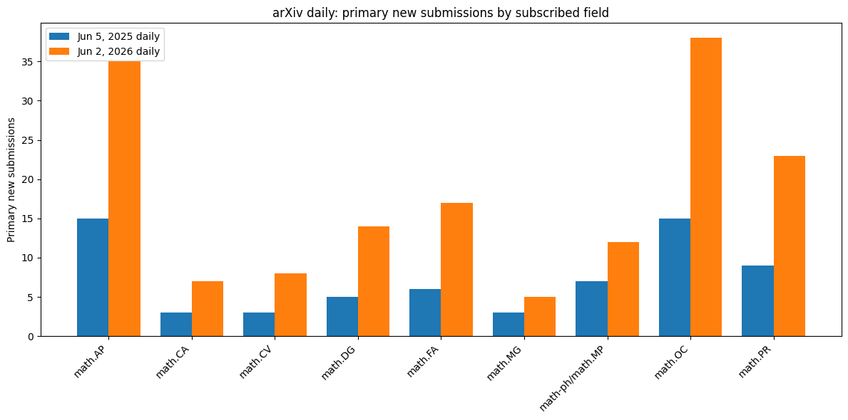
The apparent doubling was a one-day anomaly. Looking at the full final week of May, arXiv math submissions were up about 32% YoY, not 100%.

My prediction (and it is already happening): we are entering the two-day paper era.

Day 1: solve the problem.
Day 2: verify the proof, write the paper, and submit.

[Paata Ivanisvili @PI010101]

arXiv math daily submissions have more than doubled since 2025

[Paata Ivanisvili @PI010101]

New paper with Rupert Frank on https://t.co/5BplQcnkv7

We settle the problem of finding the sharp constant in the log Sobolev
inequality on the n-cycle for all n ≥ 4, by showing that it is equal to half of the spectral gap.

The question goes back to Diaconis–Saloff-Coste (1995). Even n=2k were settled by Chen–Sheu (2003); n = 5 by Chen–Liu–Saloff-Coste (2008); odd n ≤ 21 by computer-assisted proofs of Faust–Fawzi (2021). The n = 3 cycle is the exceptional case.

[Paata Ivanisvili @PI010101]

Academia is one of the few places where, despite all its imperfections, a person could still rise mostly through talent, curiosity, and hard work (example: Ramanujan) — not only through luck, wealth, family connections etc.

But what happens if access to extremely powerful AI assistants becomes the new dividing line?

The news about “superhuman AI” is scientifically exciting. But socially, it raises difficult questions — especially for gifted children from poor backgrounds who may not have access to frontier models.

[Paata Ivanisvili @PI010101]

@ElliotGlazer Someone should really give him access to frontier models. In many cases, with a bit of experimentation using LLMs, one can improve these constants quite substantially. For example, with a little play, one can already get something like n^1.0318499…

[Paata Ivanisvili @PI010101]

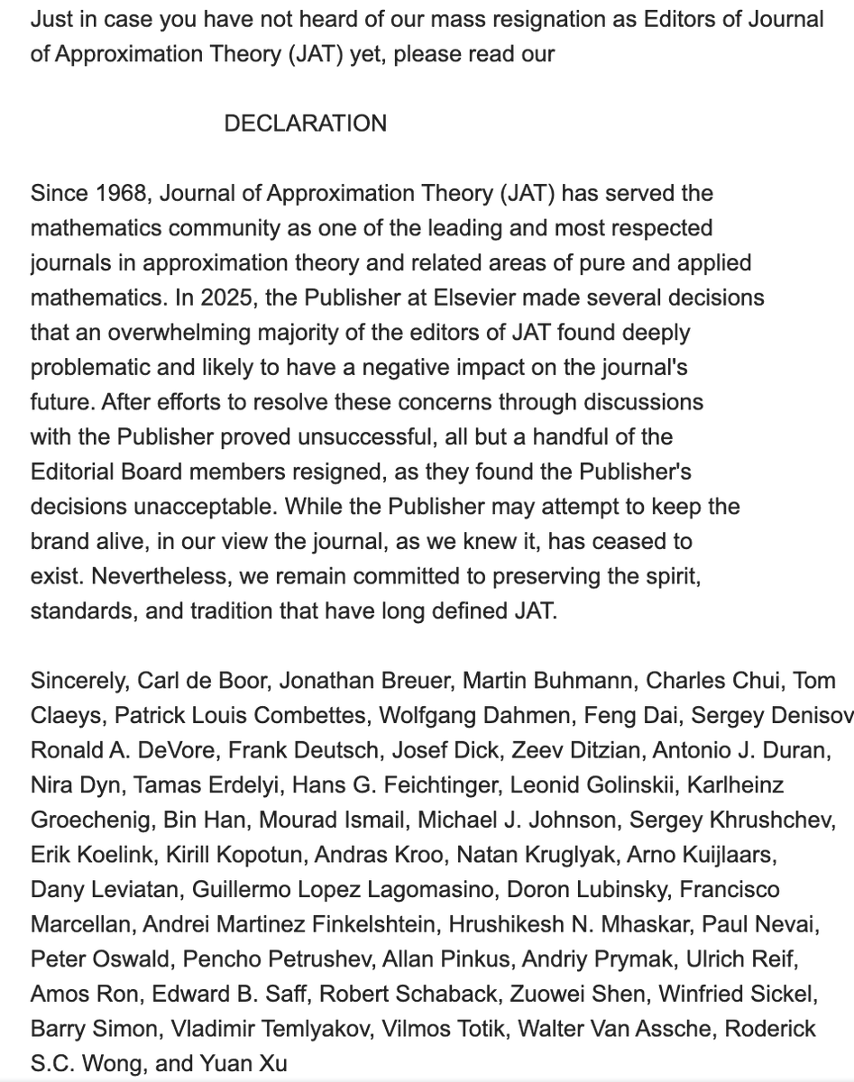
A remarkable moment in mathematics publishing: almost the entire editorial board of the Journal of Approximation Theory has resigned simultaneously, declaring that “the journal, as we knew it, has ceased to exist.”

[Paata Ivanisvili @PI010101]

Grateful to share that my NSF DMS grant has been awarded.

The project studies functions of many yes/no variables and their continuous analogues, with connections to high-dimensional probability, learning theory, data science, and quantum computation. The goal is to understand approximation, randomness, boundary structure, and sharp inequalities.

Many thanks to NSF and DMS for their support.

@NSF_MPS #DMSFunded

[Paata Ivanisvili @PI010101]

Déjà vu effect in LLMs

I was working on a problem, call it Problem A. At some point I managed to reduce it to another problem, call it Problem B, and then solve B.

Problem B is interesting in its own right and can naturally be asked in a more general setting, depending on a parameter (t). For my application to Problem A, I only needed the case (t=2), so I never seriously thought about the other values. My feeling was that, with enough time, perhaps one or two weeks, I could probably solve problem B for other (t)'s as well.

Now comes the interesting part.

I gave Problem B to an LLM and asked: for which values of (t) can you solve it?

It produced a solution only for (t=2). The solution looked “different” from the published one: different language, different framing, no citation to my work. But after looking more carefully, I think it is essentially the same solution, just translated into another language. This is not completely trivial to recognize unless one knows the problem well.

When I asked the LLM to solve Problem B for other values of (t), it could not.

I have seen this phenomenon in other examples as well. Sometimes, when an LLM appears to produce a new solution to a problem, I worry that what is happening is more subtle: the problem may already have been solved somewhere, perhaps in a hidden or disguised form, and the model is showing us the same solution from a different angle.

This “déjà vu effect” makes it quite hard to judge novelty in some AI-assisted mathematics.

[Paata Ivanisvili @PI010101]

@roydanroy By the way I am curious to know how is co-matheamtician doing with optimization in BMO problem (public tier-4)?

[Paata Ivanisvili @PI010101]

I agree that bringing in Lean would be very valuable, especially for disputed benchmark problems. My only worry is making formalization an upfront requirement for contributors.

When I contributed my BMO optimization problem — public Tier 4 — if I had also been required to formalize the solution in Lean, I probably would not have contributed it. The extra time cost would have been too high.

[Paata Ivanisvili @PI010101]

@kfountou Totally agree, strange times indeed 😄

[Paata Ivanisvili @PI010101]

New referee standard:
‘We reject the paper because the result is now routine with the help of LLMs’ 😄

[Paata Ivanisvili @PI010101]

@kfountou Yes, this is happening now. I’d have no objection to such a referee comment--provided they include a chat transcript (one prompt or many) that independently reproduces the same result with a complete, rigorous proof… not just copy-pasting my publicly available 10-page proof.

[Paata Ivanisvili @PI010101]

What will mathematics look like 7 years from now? I’m really curious to hear your brief opinion.

[Paata Ivanisvili @PI010101]

Still excited about these 3Blue1Brown-style videos generated by AI. Here’s a beautiful illustration of a classic analysis problem:

Let f be convex, nonnegative on [0,∞), with f(0)>0 and f(x)→0 as x→∞. Place a light source at (0,b) with 0<b<f(0). Rays reflect off the graph of f and the x-axis following the usual laws of optics.

Question: can any ray escape to +∞, or do all trajectories eventually come back? Prompt to video https://t.co/4MbPLzEilH

[Paata Ivanisvili @PI010101]

Brownian motion in 2D by Grok 4.3 (beta)

https://t.co/YYFT3fua2d

[Paata Ivanisvili @PI010101]

I asked Grok 4.3 (beta) to generate Beamer slides (PDF) for a talk based on my paper https://t.co/oRZnHw6QZx

Honestly impressed--especially with how it extracted and presented the mathematical content. I’d tweak a few details, but ~85% of the job is already done very well.

Full chat, prompt and slides: https://t.co/M0rgc3dREJ

[Paata Ivanisvili @PI010101]

@octonion Right. The beauty of a sharp bound is that it marks the endpoint—there’s simply nothing left to improve.

[Paata Ivanisvili @PI010101]

We’ve just finished revising the paper to incorporate the Bellman function suggested by Grok 4.20: https://t.co/pgJw9Mbcpz

I’ll say this: it’s quite rare in this field for a sharp bound (i.e., an exact Bellman function) to admit such a clean closed form. Interestingly, there are two ways to represent the solution: one via a stopping-time construction (a probabilistic approach, as Grok did), and another via an infinite series (a more analytic, Fourier-based approach). Had one pursued the latter, verifying the “two-point inequality” would have been extremely difficult.

[Paata Ivanisvili @PI010101]

Disclaimer: I had given early access to internal beta version of Grok 4.20

It found a new Bellman function for one of the problems I’d been working on with my student N. Alpay.

The problem reduces to identifying the pointwise maximal function U(p,q) under two constraints and understanding the behavior of U(p,0).
In our paper https://t.co/pgJw9MaEA1 we proved U(p,0)\geq I(p), where I(p) is the Gaussian isoperimetric profile, I(p) ~ p\sqrt{log(1/p)} as p ~ 0.

After ~5 minutes, Grok 4.20 produced an explicit formula U(p,q) = E \sqrt{q^2+\tau}, where \tau is the exit time of Brownian motion from (0,1) starting at p. This yields U(p,0)=E\sqrt{\tau} ~ p log(1/p) at p ~ 0, a square root improvement in the logarithmic factor.

Any significance of this result? It will not tell you how to change the world tomorrow. Rather, it gives a small step toward understanding what is going on with averages of stochastic analogs of derivatives (quadratic variation) of Boolean functions: how small can they be? 

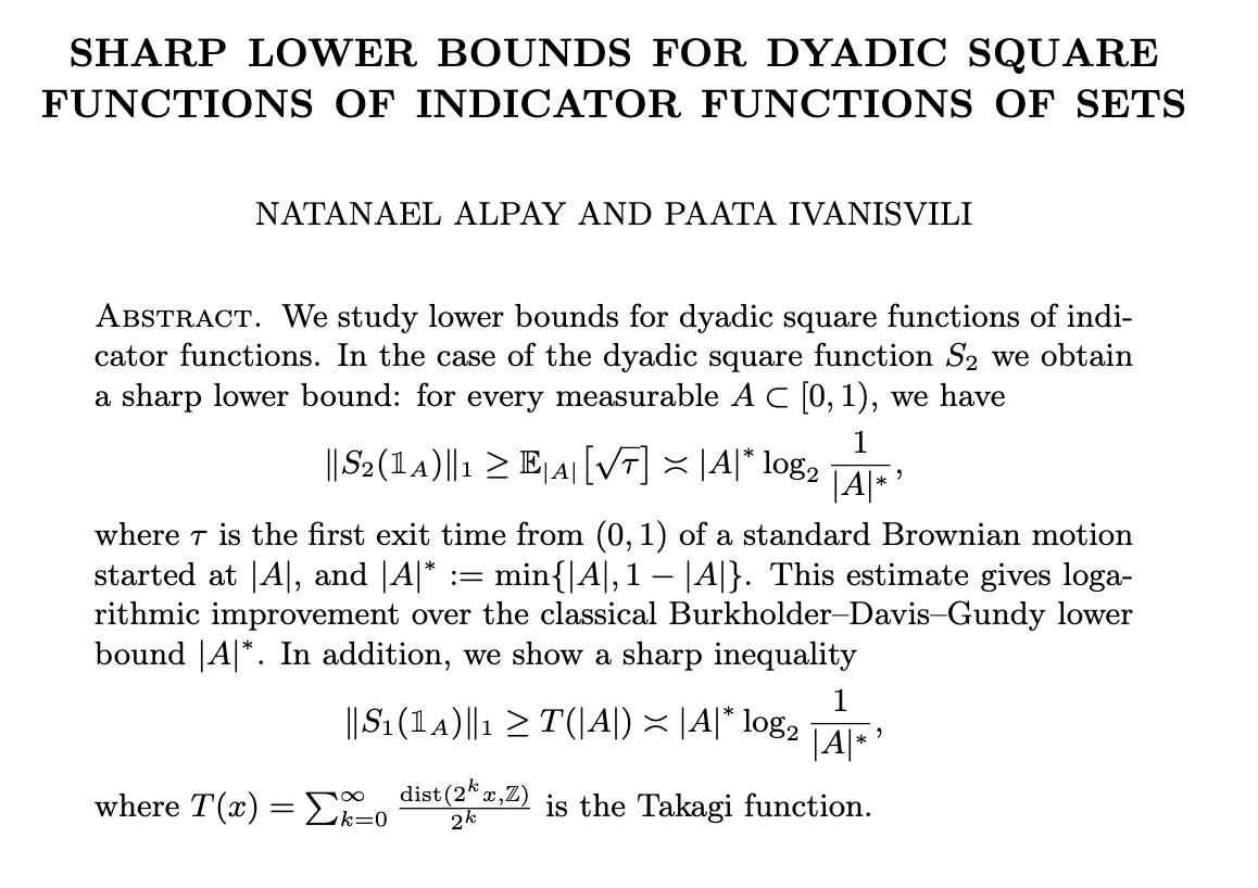
More precisely, this gives a sharp lower bound on the L1 norm of the dyadic square function applied to indicator functions 1_A of sets A \subset [0,1].
In my previous tweet about Takagi function, we saw that the sharp lower bound on ||S_1(1_A)||_1 miraculously coincides with Takagi function of |A| which (surprisingly to me) is related to the Riemann hypothesis. Here, we obtain a sharp lower bound on ||S_2(1_A)||_1 given by E \sqrt{\tau}, where Brownian motion starts at |A|. This function belongs to the family of isoperimetric-type profiles, but unlike the fractal Takagi function, it is smooth and does not coincide with the Gaussian isoperimetric profile.

Finally, in harmonic analysis it is known that the square function is not bounded in L^1. The question here was more about curiosity: how exactly does it blow up when tested on Boolean functions 1_A.  Previously, the best known lower bound was |A|(1-|A|) (Burkholder—Davis—Gandy). In our paper, we obtained |A| (1-|A|)\sqrt{log(1/(|A|(1-|A|)))}. This new Grok’s Bellman function gives |A| (1-|A|) \log(1/(|A|(1-|A|))) and this bound is actually sharp.

[Paata Ivanisvili @PI010101]

When one first looks at Condition 1, it is not immediately clear how to proceed. A natural starting point is to pass to the local form of the inequality: send a to zero, perform a Taylor expansion, and then solve the resulting differential inequality as an equality. In this case, one is led to the backward heat equation. Coming from an analysis background, the standard approach is to solve this equation on a cylinder via Fourier series (see the formula for u(p,t) on page 22). However, this turns out to be a dead end: once the solution is expressed as an infinite series, it becomes nearly impossible to return and verify the original global Condition 1.

What we were missing was a different representation of the solution--namely, one in terms of stopping times. This perspective comes from stochastic PDEs, which is not my primary area, but is likely standard in SPDE literature. The key insight is that this stopping-time representation (via Brownian motion and its Markov property) allows one to verify the global Condition 1. This approach is particularly elegant and is described in detail in Section 4 of the revised manuscript.