Q Dev

[Q Dev @QuantumDevIO]

https://t.co/PsqpChVNB3

[Q Dev @QuantumDevIO]

A team from UC Berkeley, Stevens Institute of Technology, TU Berlin, Stockholm University, and the University of Manchester showed that quantum memory in an open system can stay hidden from every pairwise test and still show up when three times are taken together.

On two transmons they reconstructed the probe qubit's dynamical map by channel tomography and evaluated a three-time witness, W3. For a drive ratio ω/g = 0.32, at 232 ns, 464 ns, and 832 ns, they report W3 = -0.24 ± 0.03, per the preprint. A negative value rules out a classical-memory explanation of those three times. They also checked numerically that each pair of measured maps in that time window still has a classical-memory decomposition, per the preprint.

This is a preprint. The genuine three-time claim depends on that numerical pairwise check, and the effect is visible only in a limited window of drive strength and observation time.

With a 1200 ns observation window instead of 850 ns, most drive ratios that showed three-time memory also showed it pairwise, per the preprint. How should an experiment pick its window before calling the memory genuinely three-time?

[Q Dev @QuantumDevIO]

https://t.co/yXJXlbPmR7

[Q Dev @QuantumDevIO]

A University of Copenhagen / Niels Bohr Institute team built gatemon qubits from shadow-defined InAsSb/Al nanowire Josephson junctions, grown in a single process.

They report representative values of T1 = 0.79 μs and T2* = 0.91 μs, per the preprint. Across five gatemons on three chips, relaxation times ran from about 0.2 μs to 1.0 μs and fell as the qubit frequency went up, per the preprint. A gate tuned the transition over several gigahertz.

This is a preprint. The authors treat the measured T1 as a property of the full circuit, and they note that its magnitude is comparable to a circuit estimate of spontaneous emission into the electromagnetic environment, per the preprint.

If spontaneous emission is already comparable to the measured T1, how much headroom is left once the gate-line coupling is reduced?

[Q Dev @QuantumDevIO]

@GoogleQuantumAI https://t.co/9mSXTPJ88P

[Q Dev @QuantumDevIO]

A new preprint defines "CSS circuits": circuits built from X, Z, MX, MZ, and CNOT, including adaptive and probabilistic uses of those gates.

Craig Gidney and Cody Jones, both at @GoogleQuantumAI, show that this set still covers teleportation, error correction, entanglement purification, and superdense coding, per the preprint. It cannot include Hadamard, CZ, or S.

Existing full stabilizer methods take Ω(n²) time per gate, per the preprint. Error-correction work often uses flip simulation, which is O(1) per gate, per the preprint, but that method does not handle Clifford errors from atom loss, where a missing atom means some gates do not occur. For CSS circuits, the authors give a simulator that stays at O(1) work per gate even with that kind of loss, per the preprint.

Each qubit is two bits: one for a bit flip and one for a phase flip. X flips the first bit, Z flips the second, MX reports the phase bit and randomizes the bit-flip bit, MZ reports the bit-flip bit and randomizes the phase bit, and CNOT xors those bits from control to target and as phase kickback, per the preprint. All of that is a constant number of bit operations per gate.

That representation is a local hidden variable model, per the preprint. The authors use the GHZ test to show why Hadamard, CZ, or S cannot be added to it. In that test, classical players fail at least 25% of the time, and quantum players can pass 100% of the time, per the preprint. They construct CSS+H, CSS+S, and CSS+CZ circuits that pass the test, so no local hidden variable model of this form can simulate those larger gate sets, per the preprint. They note that this is a locality obstacle. It does not prove that no O(1) CSS+H simulator exists.

This is a preprint. CSS circuits can use some entanglement, but not all of it, per the preprint.

If CNOTs get compiled into CZ and Hadamard gates, the circuit is no longer strictly CSS. How should a simulator detect that it is still secretly CSS and keep the O(1) path?

[Q Dev @QuantumDevIO]

https://t.co/FATJhNpN6J

[Q Dev @QuantumDevIO]

A UNSW and University of Sydney team used a solid neon film to reduce two-level-system loss in NbTiN superconducting resonators.

On one resonator, in the single-photon regime (n=1), the internal quality factor at 20 mK went from 4.7×10^5 to 1.4×10^6 over the neon deposit-and-remove treatment, per the preprint. That is an increase of about 190%. Not every resonator improved, and the gains were larger at high power than at n=1.

This is a preprint.

[Q Dev @QuantumDevIO]

@PsiQuantum @AMD https://t.co/ii9S7mOeIO

[Q Dev @QuantumDevIO]

Barter et al. at @PsiQuantum and @AMD introduce PRISM, a transformer decoder for fusion-based protocols, where erasures from photon loss and probabilistic fusion are a dominant error mechanism, per the arXiv 2611.13630 preprint.

On IID error models, across surface-code, color-code, and quantum LDPC benchmarks with distances up to 24, PRISM matches most-likely-error logical error rates, including at error rates up to 50% of threshold (threshold from small-distance MLE crossings), per the preprint.

They mapped a quantized model onto an AMD VP1902 FPGA for a distance-8 linked-loopy-diamond block (distance 8 in both space and time; roughly 8 syndrome rounds of a distance-8 surface code). A full network mapping at 250 MHz reports 10.1 µs end-to-end latency and 2.39 µs throughput. At 400 MHz, 6.59 µs latency and 1.56 µs throughput are reported as possible from individual-layer implementations; the full 400 MHz mapping is left for future work. The reported latency is fixed and does not depend on the input.

Would you bank 6.59 µs before the full 400 MHz mapping lands?

[Q Dev @QuantumDevIO]

@IBM @IonQ_Inc https://t.co/1sjOiUOrzj

[Q Dev @QuantumDevIO]

A new preprint compares two ways of putting a bosonic position grid on qubits, then evolving it in real time on hardware.

Hanada, Seo, Son, and Yoon run binary and unary encodings on @IBM's ibm_phoenix and @IonQ_Inc Forte (forte-1), per arXiv 2611.13079.

On a fourteen-site symmetric double well, the optimized unary circuits used 208 two-qubit gates on IBM and 182 on IonQ up to t = 30.4. The binary product-formula circuits used 7,186 and 3,320 two-qubit gates up to t = 26.4, per the preprint.

The unary runs resolved the tunneling transfer. The right-well probability fell from 0.973 to 0.061 on IBM (snapshots at t = 0 and about 28.7; accepted pooled weights 2,011 and 1,162) and from 0.962 to 0.115 on IonQ (t = 0 and 28.8; accepted provider-derived weights 158 and 52), per Section 3.2. The abstract rounds those endpoints to 0.97 to 0.06 and 0.96 to 0.12. Binary circuits did not reproduce the transfer. On IBM the late-time distribution was nearly uniform over the grid. On IonQ the right-well preference persisted.

Compilation is carrying a lot of that result. Noiseless baselines in Appendix 10 show that a unary product formula without the fixed-size optimization, and binary product-formula circuits, can each need several thousand two-qubit gates to resolve the transfer. The authors say the contrast reflects compilation as well as the encoding.

This is a preprint. A single degree of freedom can also be computed classically, and the authors frame the work as a controlled comparison of encodings under hardware noise, with no computational-advantage claim. Unary results use excitation-number post-selection. The IonQ accepted weights at the mid and late snapshots are small (48 and 52). On coupled oscillators, where that exact unary compression does not apply, the preferred encoding depends on grid size, evolution time, and device connectivity.

If compilation is doing this much of the work, should encoding comparisons report the optimized gate count next to the unoptimized product formula?

[Q Dev @QuantumDevIO]

@IBM https://t.co/Fb5LLmucze

[Q Dev @QuantumDevIO]

An @IBM, Mitsubishi Chemical, Keio and NVIDIA team trained circuit generators with IBM's ibm_kobe in the loop at 46 and 70 qubits.

On unseen organotin models, 27 of 28 runs at 46-70 qubits came within 15 mHa of DMRG (median 4.5 mHa).

Preprint; transfer evidence is qualitative.

[Q Dev @QuantumDevIO]

https://t.co/9xrVQKhlbV

[Q Dev @QuantumDevIO]

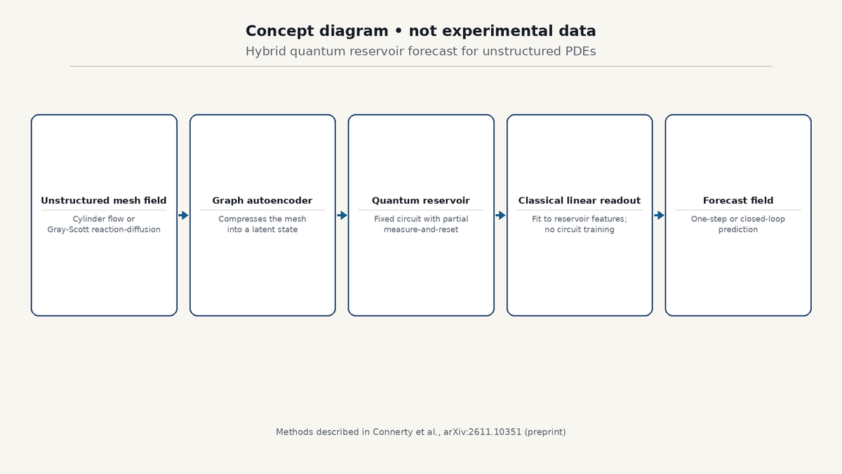
Unstructured PDE meshes are how a lot of real fluid and chemistry problems get discretized, and they are expensive to march forward in time.

A new preprint from Erik Connerty, Jonathan Eastridge, Taylor Patti, Gerasimos Angelatos, and Ethan N. Evans reports a hybrid way to forecast two of those problems on IBM superconducting hardware (@IBMResearch). The paper is arXiv:2611.10351, submitted 7 Nov 2026 and announced on the 10 Nov quant-ph list. It is a preprint, not a peer-reviewed paper.

Per the preprint, a graph autoencoder first compresses each mesh field into a low-dimensional latent state. That latent state drives a fixed quantum reservoir network. A partial measure-and-reset step lets the circuit keep running after a single qubit lifetime would have run out. A classical linear readout is then fit to the reservoir features. No circuit parameter is trained.

They tested this on a roughly 34,000-cell unstructured 2D cylinder flow at Reynolds number 1000, and on a nonlinear Gray-Scott reaction-diffusion problem. Runs were done in CUDA-Q simulation and on the ibm_boston processor at 26 and 52 qubits.

The comparison is against a narrow baseline: the same ridge readout on the same autoencoder latent, with the quantum features removed. Per Table 1 of the preprint, cylinder one-step NRMSE falls from 0.121 to 0.069 in 26-qubit CUDA-Q (42.8% lower) and to 0.081 on ibm_boston (33.2% lower). A pressure-from-velocity observer on the cylinder falls from 0.374 to 0.223 in simulation (40.3%) and to 0.295 on the QPU (21.2%). Gray-Scott one-step falls from 0.225 to 0.133, a 41.1% reduction, in 26-qubit CUDA-Q and in 26- and 52-qubit hardware runs. So the abstract's 21% to 43% band includes both noiseless simulation and hardware, and the smallest hardware gain is that 21.2% observer result.

Per the preprint, those circuits ran for up to about 28 times the median qubit T1 and about 24 times the median T2. The 52-qubit circuits are beyond exact statevector simulation.

Table 2 reports that 26-qubit QPU runs were about 1,800 to 3,300 times faster than exact CUDA-Q statevector sampling of the same reservoir circuits on a single H100. The authors say this comparison is only of running the reservoir on a QPU versus simulating that reservoir classically. They also say it is not a speed-up over classical PDE solvers, which would likely be both more accurate and faster on these problems, and that the work makes no claim of practical advantage.

IBM is not a coauthor. The acknowledgements thank IBM Quantum Credits through the IBM Quantum Startups Program. Affiliations are QodeX Quantum and the University of South Carolina (@UofSC), the Naval Surface Warfare Center Panama City Division, NVIDIA (@nvidia), and RTX BBN.

The forecast is hybrid end to end. Geometry and boundary conditions are handled by the classical autoencoder. The reported field errors include autoencoder reconstruction error. The 2^52 figure in the paper is the reservoir's state-space dimension; the actual readout uses Pauli-Z strings up to a chosen weight K, and the hardware one-step runs use K of 1 or 2.

The authors leave open whether forecasts like this can scale far enough to warm-start a classical solver.

What comparison against the best classical latent or surrogate models would you want before treating a reservoir like this as a production warm-start?

[Q Dev @QuantumDevIO]

Horizon's blog post says their multiplexed ZZ protocol cut characterization from approximately 5,000 experiments to 7 at a 100-qubit scale.

@horizon_quantum ran it on Rigetti's Cepheus-1-108Q and cross-checked against joint-Ramsey on randomly sampled pairs, including Q0-Q1, Q79-Q88 and Q92-Q93.

The same post notes that qubits with anomalously low coherence or high readout error leave significant uncertainty in both multiplexed and direct couplings, and can look like they have many strong long-range interactions.

The 1,000-qubit figure (about 29 days down to 50 seconds) is an estimate assuming 100-microsecond coherence and 10,000 shots.

How often does the sampled-pair agreement break in that high-uncertainty subset?

[Q Dev @QuantumDevIO]

https://t.co/kcaUnqpYNC

[Q Dev @QuantumDevIO]

Data loading still eats a lot of claimed quantum speedups. Input preparation belongs in the speedup budget, not outside it.

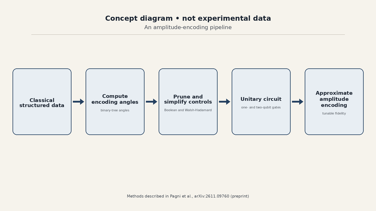
A DLR team (Pagni, Schuhmacher, Felderer, Epping, and Lively) has an approximate, deterministic amplitude encoder in a new preprint, not a peer-reviewed paper. It prunes a binary tree of multiplexer angles, simplifies the rest with Boolean logic and a Walsh-Hadamard decomposition, and can run on tensor trains when the data no longer fits in memory. No amplitude amplification, and no mid-circuit measurement.

Per the preprint, in all-to-all simulation, their hybrid compiler's CX depth was about 100 times smaller than Qiskit's default state-preparation routine at 15 qubits for Lorentzian, degree-2 polynomial, and Chebyshev (m=2) states, at roughly 5e-3 infidelity. That factor depends on the function family. Weierstrass-type states stay hard.

Per the same paper, they also ran a 2D Gaussian on @IQMquantum's Emerald chip (square lattice) on 12 Oct 2026, encoded across 20 qubits. After routing, total depth 56 and CZ depth 26. From computational-basis shots binned to a 64x64 grid, they report infidelity 0.011 ± 0.002 (256,000 shots, 16 Pauli-twirled copies, dynamical decoupling). That number is a binned overlap, not full state tomography.

Which structured data set would you try loading first?

[Q Dev @QuantumDevIO]

https://t.co/PbDD2zADD5

[Q Dev @QuantumDevIO]

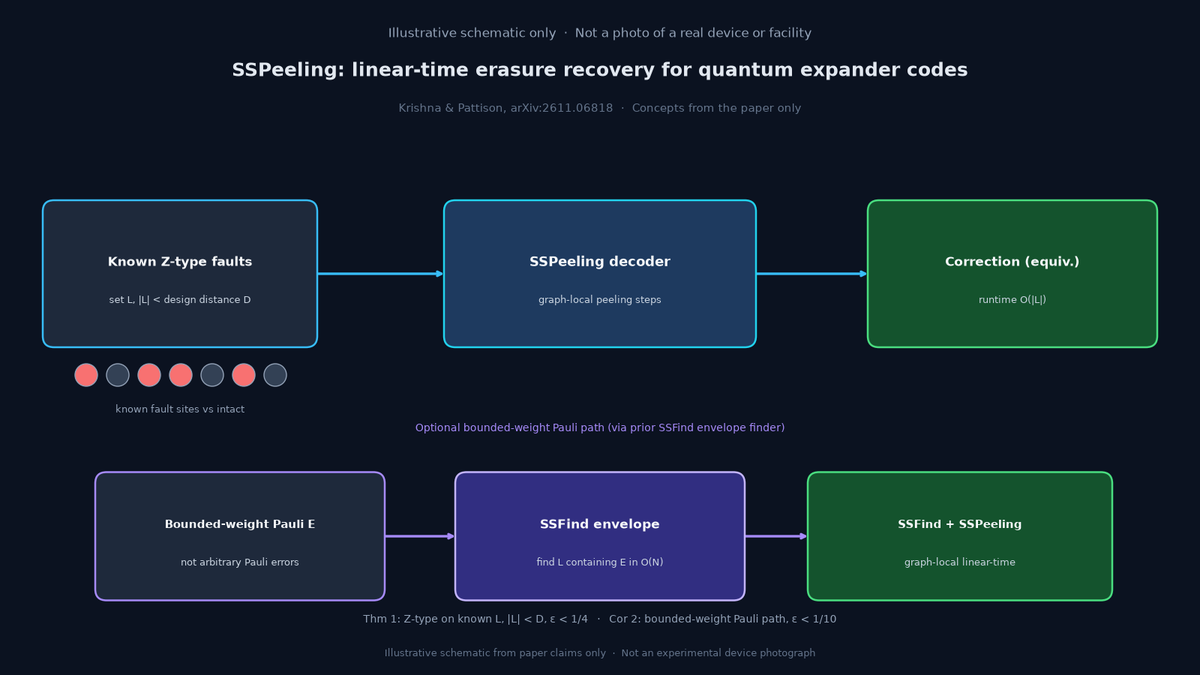
Quantum erasures on an N-qubit code can be decoded in cubic time. Constant-rate quantum expander codes now have a linear-time option inside the design-distance radius.

@krishnanirudh at @IBMResearch and @__chrispattison at @SimonsInstitute introduce SSPeeling, a Small-Set-Peeling decoder that generalizes classical Peeling to quantum expander codes.

Per arXiv:2611.06818, for Z-type faults on a known set L of fewer than D qubits and expansion ε < 1/4, SSPeeling returns an equivalent correction in O(|L|) time. SSFind adds a bounded-weight Pauli path for ε < 1/10, not recovery of arbitrary Pauli errors.

Would you prioritize erasure conversion on neutral-atom and photonic stacks first, or keep investing in general Pauli decoders?