Alejandro Santiago

.

[Mustafa @oprydai]

study trigonometry before calculus.

otherwise you’re walking into motion blind.

• sine/cosine → waves, circles, oscillations
• tangent → slope before derivatives
• unit circle → angles become coordinates
• identities → algebra for rotating systems
• vectors → components, force, velocity, fields

calculus explains change.
trigonometry explains the geometry of that change.

without trig, calculus becomes symbol pushing.
with trig, you start seeing motion.

[Strace @straceX]

i somehow missed that C23 added checked integer arithmetic.

would have saved me from writing the same overflow helper for the 20th time.

[Vivek Galatage @vivekgalatage]

Understand the impact of branching

https://t.co/04FZLB6Hl4

[Ryan Peterman @ryanlpeterman]

Avi Wigderson is the only person in history to have won both a Turing Award (computer science) and Abel Prize (math). I interviewed him all about his field. We discussed:

• His intuition on a proof of P vs NP
• Why we use SAT solvers for most NP problems
• Zero knowledge proofs and their impact
• Quantum computation and implications
• Math and computer science's relationship

Where to watch:
• YouTube: https://t.co/zViqAulFCo
• Spotify: https://t.co/iat08Xob17
• Apple Podcasts: https://t.co/jOYDGtGVnt
• Transcript: https://t.co/k4zS7yOhnw

Thank you to this episode's sponsors for supporting my work:
• WorkOS: makes your app Enterprise Ready with easy to use APIs to add SSO, SCIM, RBAC, and more in just a few lines of code, check them out at https://t.co/y8noBzFEem

Timestamps:

00:00 - Intro
01:08 - P vs NP
14:51 - What if you relaxed correctness
25:38 - Why NP complete problems are equivalent
30:33 - Space vs time complexity
43:06 - Why people use SAT solvers
45:53 - Randomness is a resource
55:48 - Randomness depends on computational power
01:21:20 - Zero knowledge proofs and their significance
01:38:30 - Quantum computation and why it matters
01:56:24 - Math vs computer science
02:08:16 - Major breakthroughs and his experience
02:12:31 - Advice for his younger self
02:14:48 - Outro

[Mathematica @mathemetica]

This reference table pairs graphs with standard integral formulas:

>Area bounded by x-axis: Area = ∫_b^a f(x) dx
>Area bounded by y-axis: Area = ∫_c^d f(y) dy
>Area between two curves: Area = ∫_b^a [f(x) − g(x)] dx
>Volume of revolution about x-axis (disk method): Volume = π ∫_b^a y² dx
>Volume of revolution about y-axis (disk method): Volume = π ∫_c^d x² dx

Real-life applications: These formulas are used to calculate total accumulated quantities such as distance traveled from velocity curves, enclosed regions in economics and biology, and volumes of three-dimensional objects like tanks, pipes, vases, and machine parts in engineering and manufacturing.

[trish @TrisH0x2A]

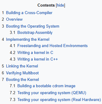
if you want to write an operating system from scratch this is the wiki almost everyone ends up using

the OSDev community has been building it since 2004

it covers everything from the first bootloader instruction to writing filesystems memory managers and drivers

the articles include real code you can compile and run yourself

the Bare Bones tutorial gets you to a kernel that boots and prints to the screen in around 100 lines

from there the wiki walks through every major piece of a real operating system

[Antonio Lupetti @antoniolupetti]

🌟Github repository
https://t.co/PSf1mKHfQy

[Mathematica @mathemetica]

The Jacobian matrix of a multivariable function f : ℝⁿ → ℝᵐ is the m×n matrix containing all first-order partial derivatives ∂fᵢ/∂xⱼ.

It linearizes the function locally and is widely used for:

> Multivariable chain rule and linear approximations
> Newton’s method for solving systems of nonlinear equations
> Gradient-based optimization in machine learning
> Forward/inverse kinematics in robotics
> Change-of-variables in multiple integrals (via its determinant)

[Mathematica @mathemetica]

L'Hôpital's Rule

For differentiable functions f and g near a (with g'(a) ≠ 0),
lim x→a f(x)/g(x) = lim x→a f'(x)/g'(x)

The diagrams illustrate the geometric meaning: as x approaches a, the ratio of the function values equals the ratio of the tangent slopes df(a)/dg(a) at that point.
This rule is applied to resolve indeterminate limit forms 0/0 and ∞/∞ by differentiating the numerator and denominator (and repeating as needed).

[Mathematica @mathemetica]

Imagine you’re trying to climb the highest peak of a mountain, but you’re forced to stay on a narrow winding trail defined by g(x) = 0. You can’t just head straight up the steepest slope by setting ∇f = 0, the mountain won’t let you.

So we invent a clever trick: the Lagrangian

ℒ(x, λ) = f(x) − ∑ λ_i g_i(x)

By solving ∇ℒ = 0, we find the exact points where the level curves of f touch the constraint boundary tangentially: the sweet spots where the gradients align (∇f = ∑ λ_i ∇g_i). These are your local maxima, minima, or saddles under the constraint.

[Mathelirium @mathelirium]

What if Your Neural Network Was Forced to Obey Physics?

Physics-Informed Neural Networks (PINNs) are neural networks trained to satisfy a differential equation by building the PDE residual directly into the loss. They emerged from a very practical problem...classical PDE pipelines can be brilliant, but they often demand heavy discretization work (meshes, stencils, stability tuning), and the method you build is usually tied to one geometry and one solver setup. A PINN flips the workflow by representing the solution itself as a smooth function uᵩ(x,t) and enforcing the physics everywhere you choose to sample the domain.

People often meet PINNs in the least helpful way...via a flashy solution plot, and almost no explanation of what was enforced to get it.

In this series we keep the enforcement visible. We pick a differential equation, represent the unknown solution as a flexible function, measure how well that function satisfies the equation across the domain, and train it to reduce that mismatch everywhere we sample.

A normal neural net learns from labels...you give it inputs and target outputs. A PINN learns from a differential equation...you give it inputs (x,t) and it gets punished whenever its output fails the PDE.

By punish we mean that the loss increases when the mismatch is large we reward it if the loss decreases as the mismatch gets smaller.

The network isn’t replacing physics, it’s becoming a flexible function that is forced to satisfy the same calculus you’d impose on any candidate solution.

The math breakdown:

We start with a PDE we want to solve on a domain Ω. Write it as

uₜ(x,t) + N(u(x,t), uₓ(x,t), uₓₓ(x,t), …) = 0 for (x,t) in Ω

A PINN replaces the unknown function u with a neural network output

uᵩ(x,t)

Now define the physics residual by plugging uᵩ into the PDE

rᵩ(x,t) = ∂uᵩ/∂t + N(uᵩ, ∂uᵩ/∂x, ∂²uᵩ/∂x², …)

If uᵩ were an exact solution, we would have rᵩ(x,t) = 0 everywhere.

We may also have data points (xᵢ,tᵢ,uᵢ) from measurements or a known initial condition. The training objective is just a weighted sum of squared errors

L(ᵩ) = L_data(ᵩ) + λ L_phys(ᵩ) + L_bc/ic(ᵩ)

with

L_data(ᵩ) = meanᵢ |uᵩ(xᵢ,tᵢ) − uᵢ|²

L_phys(ᵩ) = meanⱼ |rᵩ(xⱼ,tⱼ)|² where (xⱼ,tⱼ) are the collocation points in Ω

L_bc/ic(ᵩ) = penalties enforcing boundary conditions and initial conditions

The key technical step is that the derivatives inside rᵩ are computed by automatic differentiation

∂uᵩ/∂t, ∂uᵩ/∂x, ∂²uᵩ/∂x², …

So we can differentiate the total loss L(ᵩ) with respect to ᵩ and train with gradient descent.

This is the whole idea behind PINNs. Learn a function, but make the PDE part of the loss, so the network is trained to be a solution, not just a curve-fitter.

In the render, the main 3D surface is the network’s current guess uᵩ(x,t), drawn as a living sheet over the (x,t) plane. Hovering above is the neural scaffold...a visible graph of feature nodes and connections. The bright tension threads are the physics residual rᵩ(x,t): each thread tethers a collocation bead on the sheet up to the scaffold, and it thickens and brightens exactly where |rᵩ| is large (color encodes the sign). As training runs, those threads go slack across the domain not because we hid the error, but because the network has actually been pushed toward rᵩ(x,t) ≈ 0.

#PINNs #PhysicsInformedNeuralNetworks #ScientificMachineLearning #PDE #DifferentialEquations #Optimization #MachineLearning #AppliedMath #ComputationalPhysics

[Chao Ma @ickma2311]

David Silver RL Course (Lecture 8): Integrating Learning and Planning

AlphaGo is a beautiful example of integrating learning and planning.

🔹 The policy network gave AlphaGo intuition: which moves look promising?

🔹 The value network gave AlphaGo judgment: how good is this board position?

🔹 Monte Carlo Tree Search gave AlphaGo lookahead: simulate possible futures, expand the most useful branches, and back up value estimates through the tree

Learning gives intuition, planning gives imagination, and search turns both into action.

My note:
https://t.co/1y1P3C451c

[Avi Chawla @_avichawla]

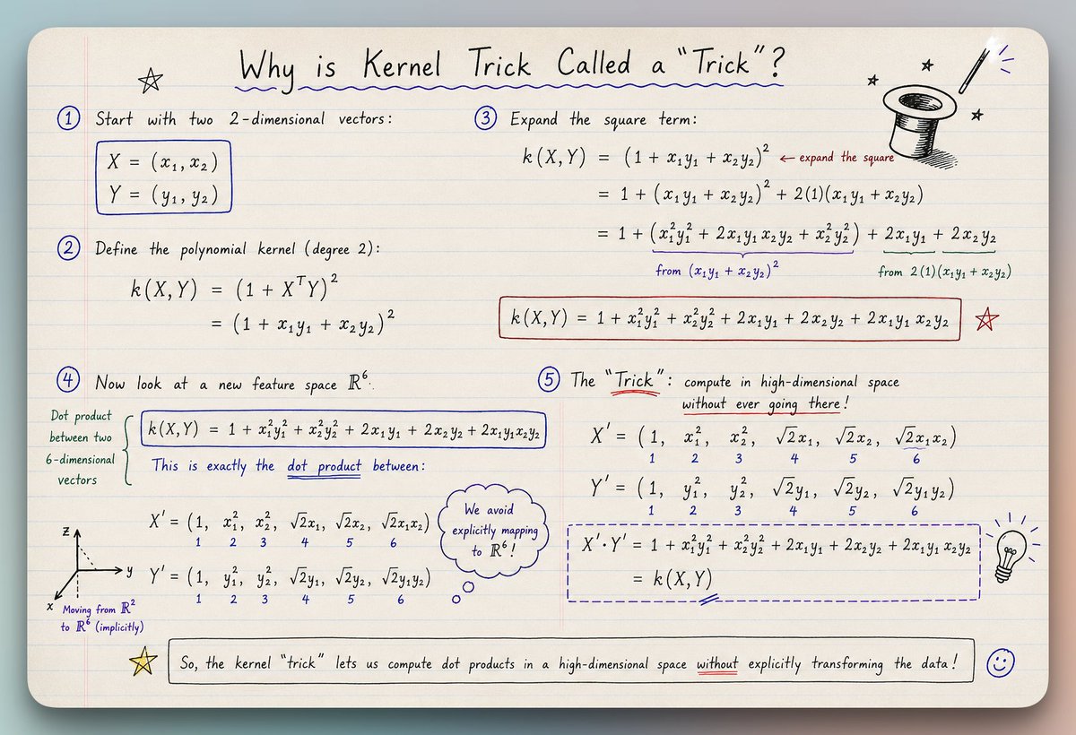
Why is the Kernel Trick called a "trick"?

(it's a popular ML interview question)

Many ML algorithms use kernels for robust modeling, like SVM, KernelPCA, etc.

The core objective of a kernel function is to compute dot products in some other feature space (mostly high-dimensional) without projecting the vectors to that space.

But how does that even happen?

Consider the image below.

Let’s assume the following polynomial kernel function:
- k(X, Y) = (1+XᵀY)².

Also, for simplicity, let’s say both X and Y are two-dimensional vectors:
- X = (x1, x2)
- Y = (y1, y2)

As shown in the image below, simplifying the kernel expression produces a dot product between the two 6-dimensional vectors.

This shows that the kernel function we chose earlier computes the dot product in a 6-dimensional space without explicitly visiting that space.

And that is the primary reason why we also call it the “kernel trick.”

More specifically, it’s framed as a “trick” since it allows us to operate in high-dimensional spaces without explicitly computing the coordinates of the data in that space.

RBF kernel is even better in this respect. It lets you compute the dot product in an infinite-dimensional space without explicitly visiting that space.

I have shared an article in the comments with a mathematical explanation of the RBF Kernel.
____
Find me → @_avichawla
Every day, I share tutorials and insights on DS, ML, LLMs, and RAGs.

[Probability and Statistics @probnstat]

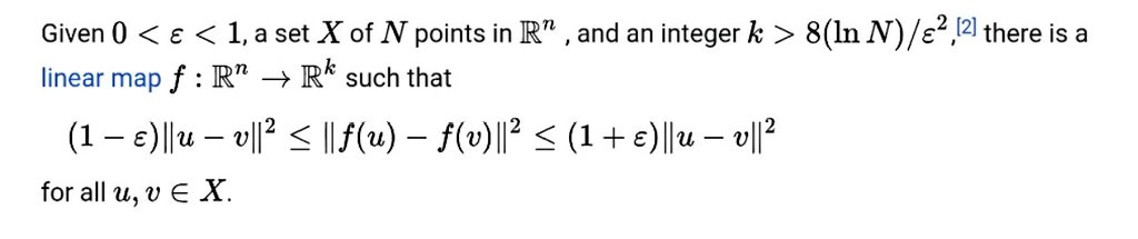
One theorem every ML engineer should know:

The Johnson–Lindenstrauss Lemma.

It states that high-dimensional data can be projected into a much lower-dimensional space while approximately preserving pairwise distances.

Why it matters:

• Explains why random projections work
• Enables scalable learning in high dimensions
• Used in embeddings, compressed learning, and ANN search
• Helps fight the curse of dimensionality

The surprising part:

You can reduce dimensions dramatically without destroying the geometry of the data.

That’s why many ML systems can operate efficiently even with massive feature spaces.

Modern representation learning is deeply connected to this idea:

Good embeddings preserve structure while compressing information.

In ML, compression is often not loss of intelligence —
it’s removal of redundancy.

[iShowCybersecurity @ishowcybersec]

1. Web Application Hacker’s Handbook
2. The Hackers Playbook 2
3. Hacking: The Art of Exploitation
4. Ghost in the Wires
5. Social Engineering: The Art of Human Hacking
6. Computer Hacking Beginners Guide
7. Kali Linux Revealed : Mastering Pen Testing Distribution
8. The Basics of Hacking and Penetration Testing
9. Nmap Network Scanning
10. Practical Malware Analysis: The Hands-on Guide
11. RTFM: Red Team Field Manual
12. Hash Crack: Password Cracking
13. Mastering Metaspoilt
14. Advanced Penetration Testing
15. Hacking: A Beginners Guide to Your First Computer Hack
16. CISSP All in One Exam Guide
17. Web Hacking 101
18. Blue Team Handbook: Incident Response Edition
19. Black Hat Python: Python
20. Gray Hat Hacking: The Ethical Hacker’s Handbook

[Mathematica @mathemetica]

Divergence - the volume density of the outward flux of a vector field.
div F = ∇ · F = ∂P/∂x + ∂Q/∂y + ∂R/∂z

Source: arrows exploding outward; ∇·F > 0
Sink: arrows collapsing inward; ∇·F < 0
Uniform flow: straight parallel arrows; ∇·F = 0

Fluids, E&M, and multivariable calculus in one picture.

[Oussama Zekri @oussamazekri_]

LayerNorm is one of the quiet tricks that makes deep networks train reliably.

Each representation centers and rescales its own features, then learns a scale and shift.

That’s LayerNorm: feature-wise normalization inside one representation!

[Jeffrey Emanuel @doodlestein]

These are so cool. We need a new kind of benchmark for visual IQ applied to these kinds of graphics. I’m still in complete disbelief that we can do this now.

[Mathematica @mathemetica]

The Fast Fourier Transform (FFT) is one of the most beautiful bridges between pure math and computer science.

It turns slow O(n²) calculations into lightning-fast O(n log n) magic; and it quietly powers your music, photos, and medical scans.

A love letter to mathematicians & CS students 🧵