Shivam Bharadwaj

Creator of Coflect. I am a Philosopher and AI professional. I love to work on advanced neural networks, neuroscience inspired AI.

[Shivam Bharadwaj @Shivam_AI]

Announcing Coflect: an agentic deep learning framework.

First public module: HILT (Human-in-the-Loop Training), realtime focus signals + in-training feedback to reduce silent failure modes like shortcut learning.

Repo:

https://t.co/MdzMtDQXsh

[Bhavin Jawade @BhavinJawade]

RL for LLMs coming full circle: REINFORCE → PPO → GRPO/DAPO → ... → back to REINFORCE?

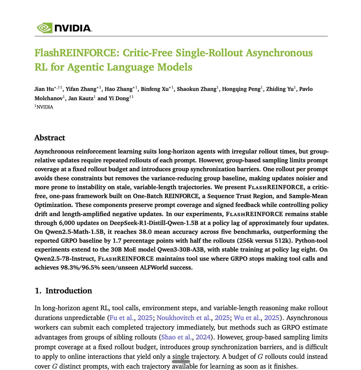
A new paper, FlashREINFORCE, asks: for long-horizon agentic RL, do we need multiple rollouts per prompt, a critic, or synchronous rollout groups?

1. What's the problem with GRPO-style training?
GRPO and variants like DAPO have become popular for RLVR. One of their biggest advantages over PPO is that they can get rid of the learned critic/value model. Instead, for every prompt, we generate K rollouts and estimate how good each response was relative to the other responses for the same prompt. No critic needed.

But we still need multiple rollouts for every prompt.

For long-horizon agentic RL, this becomes particularly generating multiple rollouts per prompt is expensive. Some agents finish quickly, while others make many tool calls, interact with environments, etc and can take much longer, slowing down advantage computation.

2. Going back to REINFORCE

REINFORCE is beautifully simple: sample a trajectory, observe reward, and use that signal for a policy-gradient update. No critic is fundamentally required. RLOO (Reinforce with leave one out) makes this particularly nice when multiple rollouts are available. For each rollout, use the mean reward of the other rollouts as its baseline: Advantage = outcomereward - average reward of the other rollouts. multiple rollouts baseline helps with variance and stable training

FlashREINFORCE wants the simplicity of REINFORCE while using only one rollout per prompt and allowing those rollouts to happen asynchronously.

But No group means no group baseline (like in RLOO/GRPO)
Their solution, instead of relying on rollouts from same prompt as baseline, use the batch mean (from diff prompts) as the baseline. Hence, still One rollout per prompt.

This still has the stale rollout problem. By the time the rollout finishes, the current policy may have moved significantly. One solution is importance sampling, like in PPO, importance ratio = probability under current policy / probability under rollout policy. But for long trajectories, correcting the entire trajectory can become extremely high variance as these ratios compound.

They proposed "Sequence Trust Region": if the sequence-level drift (staleness) is small, use the rollout with importance correction, if its high, reject the rollout and not use it for PG.

Along with these, to reduce the dominance of the longer trajectories in overall loss, they first average token level loss per trajectory and then average trajectory losses in a batch (instead of taking a normal full token batch level average).

I think Sequence Trust Region part is interesting to do longer async RL. They showed it to be stable for 6,000+ aysnc RL updates. Paper also shows that FlashREINFORCE remains competitive with GRPO-style training, despite using just one rollout per prompt.

[Vaishnavi @_vmlops]

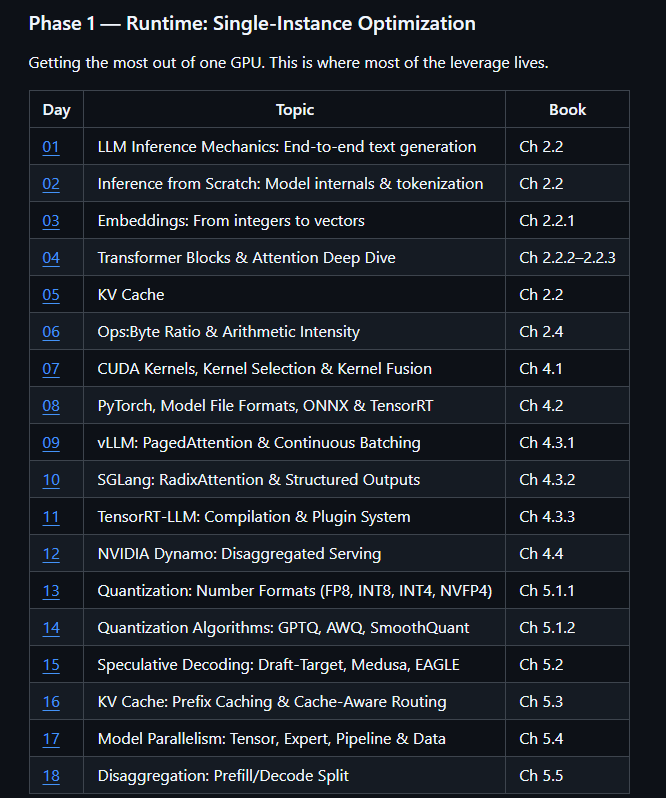
Found a genuinely solid learning resource: 100 Days of LLM Inference by @elizabetht 🔥

A structured deep-dive covering the full stack CUDA kernels → vLLM/SGLang/TensorRT-LLM → quantization → speculative decoding → multi-cloud autoscaling.

Every entry is a runnable notebook, tested on a real 2-GPU home-lab cluster

[Shane Legg @ShaneLegg]

My journey to develop AGI spans 25 yrs, including 10+ yrs thinking about technical & societal perspectives at Google DeepMind.
AGI is on the horizon - we need deeper understanding of its implications. To help, we've created the DeepMind Institute. https://t.co/dpc2y4IGT1

[Avi Chawla @_avichawla]

Layers of observability in AI systems, explained visually:

If an LLM app is serving real users, its input and output are not enough to debug it.

Consider a RAG pipeline where a query passes through embedding, retrieval, context assembly, and generation.

Every operation adds latency, may call a paid API, and can fail while still producing a valid-looking response.

Traces and spans provide visibility.

- A trace records the full path of one request. The Trace column runs from query to response.

- A span records one operation within that trace. The colored boxes are spans.

Each span captures:

> Query span

The input, timestamp, session identifier, and request metadata.

> Embedding span

The model, input size, latency, retries, and rate-limit errors.

> Retrieval span

The retrieved chunks, document IDs, relevance scores, filters, top-k value, and latency. Many RAG failures originate here. Without these fields, there is no evidence that retrieval selected the wrong documents.

> Context span

The context assembled from retrieved chunks, instructions, and conversation history. This catches truncated documents, duplicated chunks, missing citations, and prompts exceeding the token budget.

> Generation span

The model, token counts, time to first token, total latency, finish reason, retries, and estimated cost.

With these details, a bad response can now be traced to retrieval, context assembly, or generation.

To use this in practice, Opik already implements this observability infrastructure for LLM apps and is open source.

It captures traces and spans across LLM calls, retrieval steps, and tool executions, with latency, token usage, and cost attached to each operation.

GitHub repo: https://t.co/vahjkkfJCt

(don't forget to star it ⭐)

In Opik, every operation belonging to one request carries the same Trace ID. If the app processes 1,000 requests, it creates 1,000 traces, each containing its own spans.

This makes cost analysis more useful. Instead of aggregate spend, teams can identify the model calls, retries, or oversized prompts responsible.

Over time, changes in retrieval scores, embedding latency, or context size become visible before they turn into broader quality problems.

That said, observability is one of eight areas I would learn for building production LLM systems.

I covered all eight in the 2026 LLM Engineering Roadmap, with free and open-source resources for each one.

Read it below.

[Tom Yeh @ProfTomYeh]

Sora's Diffusion Transformer by hand ✍️ ~ 14 steps walkthrough below

Remember back in 2024 when Sora from OpenAI caused quite a sensation? This year, OpenAI shut it down. But the idea behind it, the Diffusion Transformer (DiT) that combines diffusion with a transformer, has led to the revolution in video generation models as we know them today.

Fancy tech names eventually die, but the foundational idea carries on.

So, how does DiT work?

Goal: generate a video conditioned by a text prompt and a diffusion step.

= 1. Given =

A training video, the prompt "sora is sky", and diffusion step t = 3.

= 2. Video to patches =

Divide all pixels in all frames into 4 spacetime patches. A patch spans space and time, which is how a video becomes a sequence.

= 3. Visual encoder =

Multiply the patches by weights and biases, then ReLU: one latent vector per patch. Here 4 numbers (2x2x1) become 2. In the paper, 196,608 become 4,096.

= 4. Add noise =

Sample noise scaled by the diffusion step t and add it to the latent features. You ruin the video on purpose so the model can be asked to guess what you ruined it with, the same trick as hiding a word from an LLM.

= 5. Encode conditions =

Encode "sora is sky" as [0,1,-1], encode t = 3 as [1,1], concatenate into one 5D column.

= 6. Estimate scale and shift =

Multiply that vector by weights and biases to get a scale [2,-1] and a shift [-1,5].

= 7. Apply scale and shift =

Scale the noised latent, then shift it. This is adaptive layer norm, the only place the prompt and the timestep touch the video. Conditioning is two arithmetic operations, not a separate model.

= 8. Self-attention =

Feed the conditioned latent to a query-key function to get a self-attention matrix. Value is omitted for simplicity.

= 9. Attention pooling =

Multiply the conditioned latent by the attention matrix. Patches now mix across space and time, which keeps frame 4 consistent with frame 1.

= 10. Pointwise FFN =

Multiply the attention-weighted features by weights and biases to get the predicted noise.

= 11. MSE loss gradients =

Take the difference between the predicted noise and the sampled noise from step 4. It kicks off backpropagation through every learnable parameter (red borders); encoder and decoder stay frozen (blue borders).

= 12. Denoise =

Subtract the predicted noise from the noised latent for the noise-free latent.

= 13. Visual decoder =

Multiply by weights and biases, then ReLU, back to patch size.

= 14. Patches to video =

Rearrange the patches into a sequence of frames.

Takeaway: DiT is a transformer that predicts noise. The video enters as latent patches, never pixels; the prompt and timestep enter only as a scale and a shift. Steps 4 and 11 are training, 12 to 14 are generation, the rest is the block you stack dozens of times.

💾 Save this post!

[Shivam Bharadwaj @Shivam_AI]

Added GoalLab, a flagship project, to the open source RL course.

It evolves from Q Learning → DQN → PPO → preference learning → agents → inference time reasoning.

The course also includes MiniLabs for tool using agents and inference time reasoning.

https://t.co/kuSH8WLLnb

[Sumanth @Sumanth_077]

https://t.co/8j8Vxf4r9u

[Sumanth @Sumanth_077]

The model is only one part of a coding agent!

The harness is what turns that model into an agent that can actually work through a codebase.

It decides what context reaches the model, which tools are available, how files and commands are handled, what rules apply to the task, and how the agent keeps working after every result comes back.

This is also why using the same model across two coding agents can produce very different results.

One harness might give the model better repository context, stronger tools, project-specific rules, reusable skills, or a better way to carry state across a long task. Another might expose the same model to a much simpler loop.

And harnesses are getting much broader now.

They are starting to include things like rules, hooks, skills, MCP servers, plugins, scheduled runs, multiple sessions, checkpoints, and different model or provider choices around the same agent workflow.

Cline Desktop brings a lot of that into one place. It is an open-source desktop app built around coding agents, with support for open-weight models alongside other model and provider choices.

You can connect a workspace, choose the model you want to run, keep different agent sessions going, schedule recurring work, and extend the setup with skills, MCP servers, plugins, rules, hooks, and tools.

The model can change depending on the task without changing the entire workflow around it.

That is the part I find useful here.

When we compare coding agents, looking only at which model they use misses a large part of what actually determines how the agent works.

The harness around that model matters just as much.

I’ve been testing an early build of Cline Desktop on one of the projects from my Hands-On AI Engineering repo, and the video below shows it in action.

[Shivam Bharadwaj @Shivam_AI]

The learning path is flexible. Start from fundamentals, jump directly into Deep RL, or focus on RL for LLMs and agents based on what you already know.

[Shivam Bharadwaj @Shivam_AI]

I’ve released my open source Reinforcement Learning course.

3 parts.
2 learning modes.
3 learning paths.
Hands on projects that run on Google Colab.

Built to make RL easier to enter and deep enough when needed.

https://t.co/kuSH8WLLnb

[Shivam Bharadwaj @Shivam_AI]

The projects are intentionally small enough to run on Google Colab, so you can experiment with DQN, PPO, DPO, GRPO, reasoning search, and more without expensive compute.

[Shivam Bharadwaj @Shivam_AI]

1. Three parts: RL fundamentals, modern RL, and inference time reasoning.

2. Two modes: Quick Read for intuition, Deep Chapter for depth.

3. Three learning paths plus hands on Colab projects to connect theory with implementation.

[Shivam Bharadwaj @Shivam_AI]

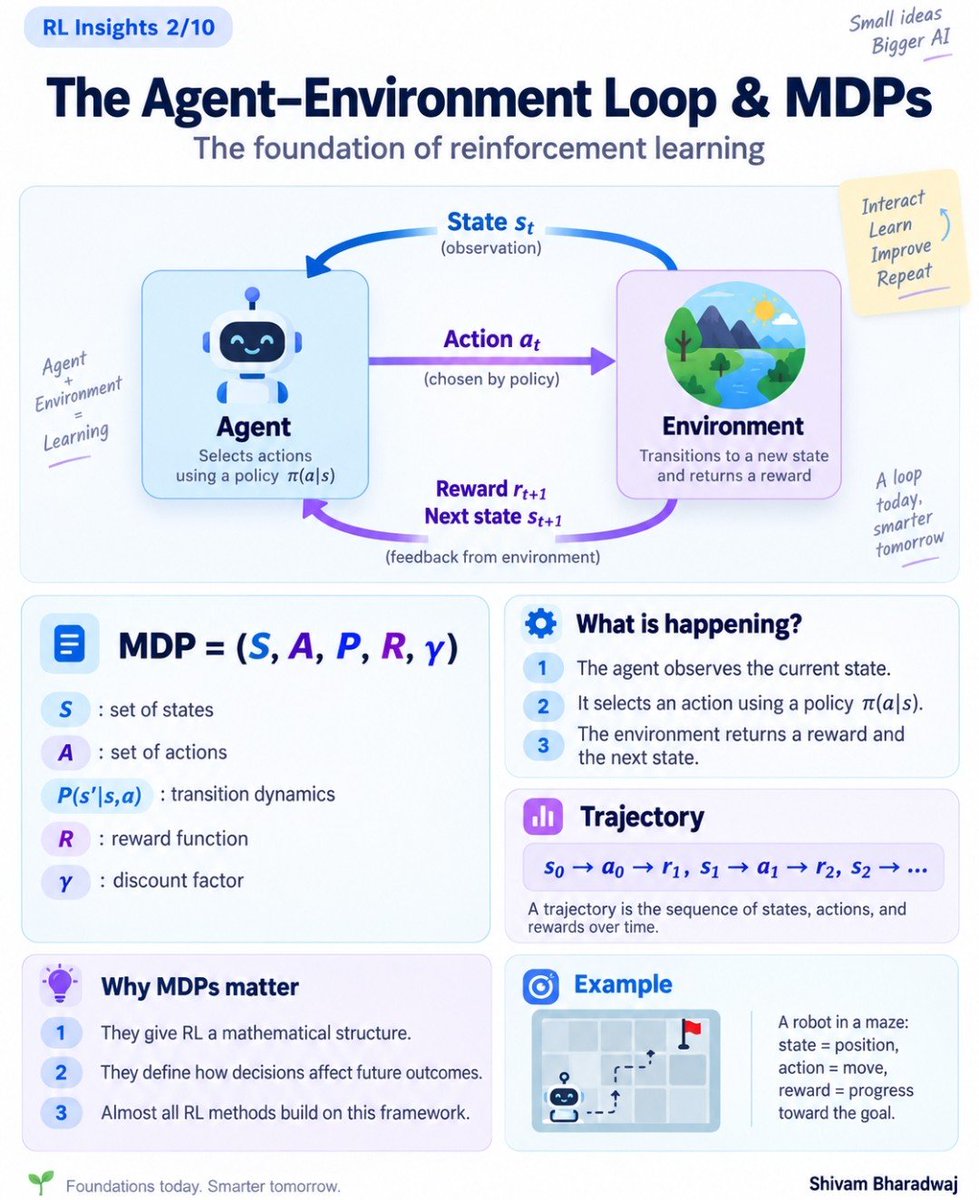
RL Insights 2/10: MDPs

Most RL problems reduce to one loop:

State → Action → Reward → Next State

An MDP formalizes it as:

M = (S, A, P, R, γ)

Understand this, and much of RL becomes easier to reason about.

#ReinforcementLearning #AI

[Kirk Borne @KirkDBorne]

AI Agents and Applications: https://t.co/Bya3yDnlaF

[448 pages. From @ManningBooks]

[Avi Chawla @_avichawla]

One architectural change can cut KV cache by 8x!

In standard multi-head attention, every query head gets its own key and value head.

So a model with 64 query heads therefore stores 64 sets of key and value vectors for every token at every layer.

Multi-query attention optimizes this. It shares one KV head across all query heads. This produces the smallest cache, although that much sharing can reduce model quality.

Grouped-query attention lies between them.

It divides the query heads into groups, with each group sharing one KV head.

In Llama 3 70B, every eight query heads share one KV head. The model stores 8 sets of KV vectors instead of the 64 that an equivalent MHA layout would need.

That makes this part of the KV cache 8x smaller. It also reduces the amount of KV data read during decoding by the same factor, assuming the remaining dimensions and precision stay unchanged.

This is part of the model architecture, so it cannot be enabled on an arbitrary MHA model with a serving flag.

And this is only one way to control KV-cache cost.

I covered GQA alongside 11 other methods in the KV Cache Engineering article. It explains which part of the cost each method reduces and whether it requires a different model architecture or only a serving-engine change.

Read it below.

[Nikki Siapno @NikkiSiapno]

𝗣𝗼𝘀𝘁𝗴𝗿𝗲𝘀 𝘃𝘀 𝗠𝗼𝗻𝗴𝗼𝗗𝗕 𝘃𝘀 𝗖𝗮𝘀𝘀𝗮𝗻𝗱𝗿𝗮.

Choosing the right database isn’t about the tool. It’s ultimately about the workload.

AWS Next Gen Stats is a great real-world example.

As Next Gen Stats evolved, it ended up using all three for different workloads. MongoDB for flexible data models and derived stats, Cassandra for predictable query latency at scale, and Postgres for analytics.

This is polyglot persistence; using different databases for different workloads instead of asking one system to do everything.

On Friday, I was in Melbourne for the NFL International Games with AWS to get a firsthand look at the engineering behind Next Gen Stats.

Next Gen Stats turns player and ball tracking data from every play into real-time statistics and insights. Behind that are some fascinating real-time data and machine learning problems.

But AWS’s database design is just one part of the architecture. Over the next three weeks, I’ll be sharing a full system design case study and video breaking down how the system works.

Learn more here → https://t.co/iXhGANzSDw

What else would you add?

——

♻️ Repost to help others learn databases.
🙏 Thanks to @awscloud for partnering with us to unpack the engineering behind Next Gen Stats, and for sponsoring this post.
➕ Follow me ( Nikki Siapno ) to improve at AI and system design.

[Shivam Bharadwaj @Shivam_AI]

RL Insights 2/10: MDPs

Most RL problems reduce to one loop:

State → Action → Reward → Next State

An MDP formalizes it as:

M = (S, A, P, R, γ)

Understand this, and much of RL becomes easier to reason about.

#ReinforcementLearning #AI

[Tom Yeh @ProfTomYeh]

Graph Convolutional Network by hand ✍️ ~ 12 steps walkthrough below

Graph Convolutional Networks (GCNs), introduced by Thomas Kipf and Max Welling in 2017, are the tool for data shaped like a graph: social networks, recommendations, biological networks, drug discovery, molecular chemistry.

I drew and calculated a simple GCN entirely by hand.

Goal: run a two-layer GCN, then a small classifier, on a five-node graph, filling in every cell yourself.

1. Given

A graph of five nodes, A to E, with edges between some of them.

2. Adjacency matrix (neighbors)

Put a 1 wherever two nodes share an edge, in both directions.

3. Adjacency matrix (self)

Add 1s down the diagonal, one self-loop per node. That is just adding the identity matrix.

4. Messages

Multiply each node's embedding by the weights and biases, then ReLU. Negatives become 0.

5. Pooling

Multiply the messages by the adjacency matrix. Each node gathers the messages of its neighbours and itself.

6. Visualize

Node A pools [3,0,1] + [1,0,0] = [4,0,1].

7. Second GCN layer

Messages again: weights, biases, ReLU.

8. Pooling again

Pool over each node and its neighbours, once more.

9. Visualize

Node C pools [1,2,4] + [1,3,5] + [0,0,1] = [2,5,10].

10. Fully connected layer

Weights, biases, ReLU. This time there are no neighbours to pool, just the node itself.

11. Linear layer

One more: weights and biases.

12. Sigmoid

Squash each score to a probability (≥ 3 → 1, 0 → 0.5, ≤ -3 → 0). That is the classification for each node.

You have just classified every node in the graph by hand. ✍️

The outputs:
A: 0 (very unlikely)
B: 1 (very likely)
C: 1 (very likely)
D: 1 (very likely)
E: 0.5 (neutral)

The takeaway: a GCN layer is two parts. The top part pools each node with its neighbours through the adjacency matrix. The bottom part is an MLP that transforms each node on its own. A transformer layer has the same two parts, with an attention matrix where the adjacency matrix was. Both matrices do one job, mixing across positions: attention over tokens, adjacency over nodes.

In my class I call the GCN the transformer's little cousin: a bit more stubborn, because its attention is fixed by the graph rather than computed from Q, K, and V. Draw the two side by side and the resemblance is hard to miss.

💾 Save this post!

#AIbyHand #GraphNeuralNetworks #DeepLearning

[Sumanth @Sumanth_077]

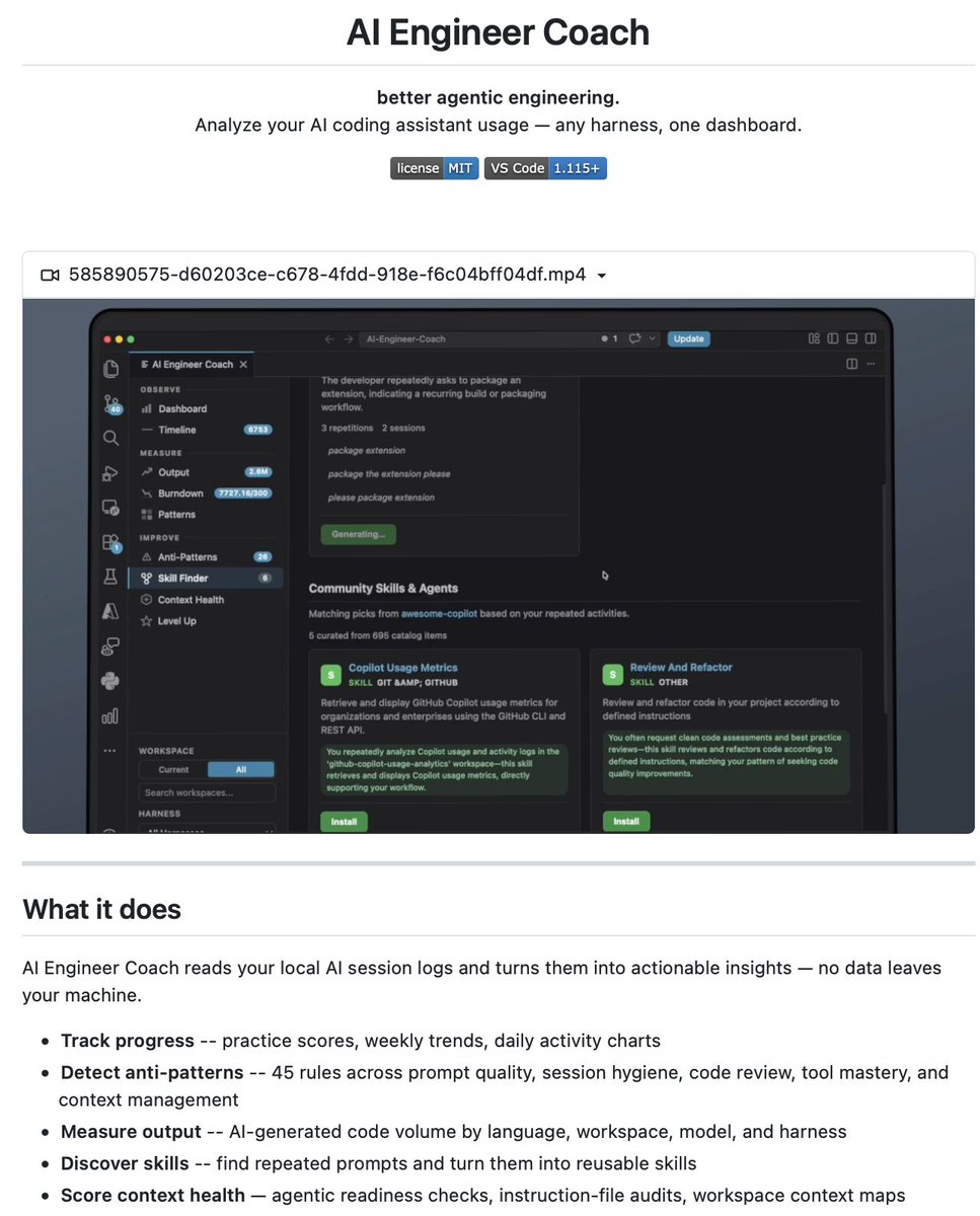
Microsoft open-sourced an AI Engineer Coach!

AI Engineer Coach is a VS Code extension that reads your local AI coding session logs and turns them into actionable insights. Works with any harness - Claude Code, Copilot, Cursor, Codex, Cline. Everything runs on your machine. No data leaves.

Most developers using AI coding tools don't know if they're actually getting better at using them. What prompts they repeat. What habits are slowing them down. What their context health looks like. This extension answers all of that.

Four layers:

1. Observe - Practice scores with week-over-week trends, daily activity charts, Gantt-style session timeline, and a screenshot gallery from your coding sessions.

2. Measure - AI-generated code volume broken down by language, model, workspace, and harness. Activity heatmaps showing your 7×24 coding patterns.

3. Improve - 45 anti-pattern rules across prompt quality, session hygiene, code review, tool mastery, and context management. Each rule comes with severity ratings and concrete actions. Skill Finder discovers repeated prompt patterns and matches them to reusable skills from the open-source catalog. Context Health runs agentic readiness checks and audits your instruction files.

4. Level Up - Personalized quizzes generated from your actual usage data. XP-based progression with Bronze to Diamond tiers. An Agentic SDLC view showing how you use AI across the full development lifecycle.

Key capabilities:

• Works with any AI coding harness in one dashboard
• 45 anti-pattern detection rules across 5 categories
• Skill Finder for repeated prompts and reusable skills
• Context Health with agentic readiness checks
• Personalized quizzes from your actual session data
• All local - no data leaves your machine
• Editable rules with live testing via Rule Playground

100% open source.

I've shared the link in the replies!

[Shivam Bharadwaj @Shivam_AI]

RL for LLMs is moving into inference.

Instead of one reasoning path:

generate → score → expand → prune

The goal becomes:

best reasoning trajectory under a fixed compute budget.

I am also building an RL course covering this from fundamentals to modern LLM reasoning.