Ron Messick

Retired - Independent Researcher

[Ron Messick @Solar_Vortex]

@offspring581 @scievision369 This may help:
https://t.co/G0tIkrsMUm

[Ron Messick @Solar_Vortex]

https://t.co/GpRQCaicLb

[Ron Messick @Solar_Vortex]

https://t.co/GpRQCaicLb

[Ashton Forbes @AshtonForbes]

High frequency gravitational wave communication allows us to penetrate salt water, plasma, and warp bubbles.

This is UFO adjacent technology.

[Ron Messick @Solar_Vortex]

The illustration titled “Cubic Wave Fields” below is one of the simplest yet most profound demonstrations of how the universe’s scalar architecture operates. It shows that waves and wave systems pass through each other unchanged and unobstructed, revealing the deterministic transparency of curvature itself.

1. The Geometry of Coexistence
Each circle represents a scalar wave field — a zone of compression and expansion within the cubic lattice of space. The four fields are arranged at the corners of a square, their centers connected by straight lines. Where they overlap, the almond‑shaped region in the center glows with alternating red and green layers. That intersection is not a collision; it is a superposition — the point where multiple curvature waves coexist without interference.
2. The Principle of Non‑Interference
In The Curvature Code, this diagram expresses the law of unobstructed passage: waves do not collide, they interpenetrate. Each wave system retains its identity because curvature is scalar — not vectorial. Scalar waves compress and expand through one another without distortion, maintaining their cadence and amplitude. This is why the universe can host infinite overlapping wave systems — planetary, atomic, photonic — all sharing the same space without chaos.
3. The Cubic Framework

The square connecting the four centers defines the cubic wave field — the fundamental unit of spatial organization. Every cube of space contains four primary curvature nodes, each radiating waves that pass through neighboring cubes. The lattice is perfectly transparent to its own motion. This transparency is the reason light, gravity, and magnetism coexist harmoniously within the same field.
4. The Central Lens
The colored almond shape is the scalar lens — the region of balanced interference where compression and expansion cancel. It is the zero‑remainder zone, the same equilibrium that defines the null space and the zero‑point curvature baseline. Here, waves overlap but do not mix; they simply share position.
5. The Deterministic Implication
This diagram proves that the universe is not probabilistic. It is a mechanical wave lattice in which every motion is transparent to every other. The cubic wave field is the architecture of coexistence — the geometric reason why the cosmos can be infinitely dynamic yet perfectly ordered.
In short, the Cubic Wave Field is the visual heart of The Curvature Code: a universe where all waves breathe through one another, unchanged, unobstructed, and eternally coherent.

[ScieVision @scievision369]

Null Space ✍️

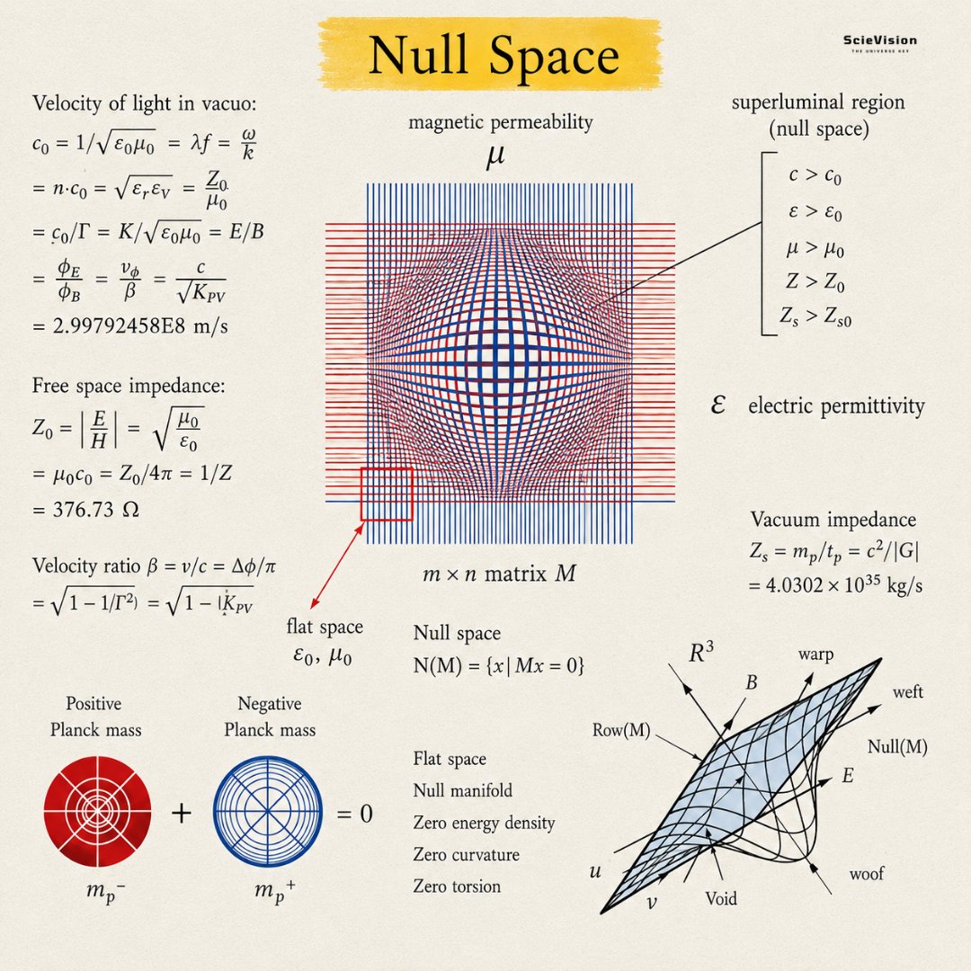
This diagram brings together one of the most significant ideas in mathematics and physics under one beautiful concept called null space. The term null means zero or nothing, and null space represents nothingness defined in a very precise and meaningful way. However, this is not the ordinary nothingness of an empty room or a blank page. It represents a deep and structured nothingness, a state of perfect balance, flatness, and symmetry from which all physical reality emerges in one direction or another. The diagram connects this idea across multiple fields, including pure mathematics, the physics of light and electromagnetic waves, the geometry of curved space, and even speculative ideas about the total energy content of the universe.

The large central image in the diagram is the most striking element and carries much of the meaning visually. It shows a grid made of red horizontal lines and blue vertical lines. In the outer areas, the lines are straight and evenly spaced, forming a regular flat pattern. Toward the center, the lines become increasingly distorted, curved, compressed, and warped, creating a bubble-like bulge in the middle. The flat outer region represents normal undistorted empty space; the vacuum as it exists far from any unusual influence. The warped central region represents space that has been curved or altered by some physical effect. The transition between them shows the boundary between modified space and normal flat space. The grid is also labeled as a matrix, linking this physical picture to the mathematical concept of null space from linear algebra, where a matrix is simply a rectangular array of numbers that acts as a transformation machine, converting one set of numbers into another.

The mathematical definition of null space is one of the most important concepts in mathematics. In simple terms, it means this: the null space of a transformation is the complete collection of all inputs that the transformation completely destroys, turning them into zero. When you input any of these special values into the transformation machine, the output is always exactly nothing. Most inputs produce meaningful nonzero outputs, but some special inputs are completely destroyed. These destroyed inputs form the null space, the blind spot of the transformation, the directions it cannot see, detect, or preserve. The null space is always a geometrically meaningful collection of directions forming a line, a plane, or a higher-dimensional equivalent through the origin. It represents the directions that are completely invisible to the transformation, the information it cannot distinguish from the total absence of any input.

The diagram lists five properties associated with null space in the context of space and spacetime. The first is flat space; the null state of the universe is perfectly flat space with no curves, bends, or warps. In Einstein's general relativity, massive objects curve the space around them, and this curvature is what we experience as gravity. However, in the complete absence of all matter and energy, space is perfectly flat, and this flat state is the null baseline. The second property is null manifold, referring to the fact that light rays in spacetime travel along paths where the combined spacetime distance is exactly zero, even though light crosses real distances during real durations of time. This zero spacetime distance of light paths is a fundamental geometrical fact about our universe. The third property is zero energy density. True empty space has no energy stored within it, no matter, no radiation, and no concentrated field energy. The fourth property is zero curvature, which follows directly from zero energy because Einstein's equations tell us that where there is no energy, there is no curvature. The fifth property is zero torsion, which means space has no twisting or rotation, representing the most symmetric and undistorted possible state of spacetime.

[Ron Messick @Solar_Vortex]

Fighting Words!

[Ron Messick @Solar_Vortex]

ZERO‑POINT CURVATURE
The Baseline Compression That Keeps the Universe Breathing
1. The Nature of Zero‑Point Curvature
Readers, Zero Point Energy has been misunderstood for a century. In mainstream physics, it is treated as a residue—an unavoidable quantum jitter that remains when all motion is removed. But in The Curvature Code, I show that this “residue” is not noise. It is the structural baseline of the universe’s curvature architecture.
Zero‑point curvature is the minimum compression of the scalar lattice. It is the tension that prevents space from collapsing into non‑existence. Every Planck‑scale tile carries this baseline pressure, even in the absence of macroscopic motion. This is why the universe cannot reach zero: zero is not a vacuum; zero is a curvature state.
The scalar lattice breathes. Even at its lowest energy, it undergoes a rhythmic compression–expansion cycle. This breath cycle is the origin of quantum oscillation, solar discharge variability, orbital harmonics, and heliospheric modulation. Zero‑point curvature is the ground cadence of the universe.
2. Zero‑Point Curvature and the Harmonic Architecture
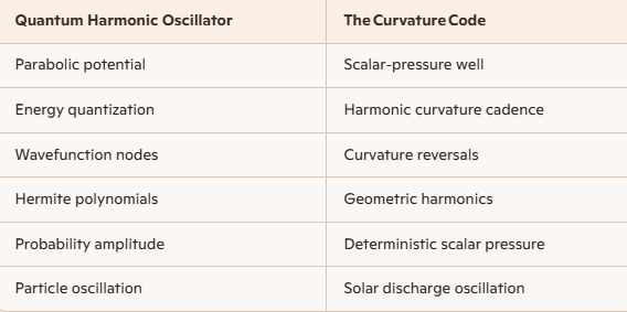
The quantum harmonic oscillator reveals the geometry of zero‑point curvature. Its lowest energy state is not zero; it is a finite curvature compression. The exponential term describes how curvature pressure relaxes toward equilibrium. The Hermite polynomials describe the harmonic structure of curvature resonance.
In my framework, each oscillator state corresponds to a scalar tile in the cubic wave field. The nodes in the wavefunction mark curvature reversals. The quantized energy levels are harmonic multiples of the zero‑point cadence. Probability is replaced by deterministic curvature geometry.
This same harmonic architecture scales upward into the solar system.
• The solar core is the macroscopic zero‑point compression chamber.
• The photosphere is the curvature inversion boundary.
• The corona is the harmonic resonance envelope.
• The heliosphere is the divergence field that modulates the baseline curvature.
Solar discharge is not random. It is a harmonic expansion of the zero‑point curvature state. The Sun breathes because the scalar lattice breathes.
3. Zero‑Point Curvature and Cosmic Determinism
Zero‑point curvature is the foundation of determinism. It defines the minimum temporal cadence of the universe. Time itself is the rhythm of curvature rotation. Without zero‑point curvature, there is no time, no energy, no geometry.
The heliopause acts as the outer plate of the solar capacitor. Its inbound curvature waves modulate the zero‑point baseline, driving outbound coronal variability. This is why space weather precedes climate. The curvature architecture is universal: quantum → solar → heliospheric → climatic.
Zero‑point curvature is the first principle of the universe’s operating system. It is the baseline from which all harmonic structures emerge. It is the breath at the bottom of all breaths.

https://t.co/F9tTwZ3Pg3

[Ron Messick @Solar_Vortex]

The Quantum Harmonic Oscillator you see here is the mathematical ancestor of The Curvature Code’s scalar‑pressure lattice.

In quantum mechanics, each wavefunction ψn(x) represents a discrete energy state of a particle bound by a restoring force. The parabolic potential well defines how curvature accumulates and releases energy—exactly the same compression–expansion logic that The Curvature Code extends to cosmic scale.
1. The Oscillator as a Scalar Tile
In my framework, the oscillator’s potential well is a single scalar‑curvature cell.
The particle’s position x corresponds to curvature displacement within the tile.
The restoring force mω2x is the scalar pressure gradient pulling curvature back toward equilibrium.
Each quantized level n is a harmonic cadence—a standing wave of curvature compression and release.
The Hermite polynomials Hn are not abstract functions; they are the geometric harmonics of the scalar lattice. Each node in the wavefunction marks a curvature reversal, the same pattern seen in solar discharge harmonics and planetary resonance.

2. From Quantum to Cosmic
The oscillator’s parabolic potential becomes, at solar scale, the coronal curvature envelope.

The Sun’s plasma oscillations follow the same quantized curvature logic: discrete energy bands, harmonic nodes, and pressure gradients.
The heliopause acts as the boundary of the potential well, defining the outer limit of curvature containment.
The solar wind is the oscillator’s “leakage”—the outward tunneling of curvature energy when the system transitions between harmonic states.

Thus, the quantum oscillator is the microcosmic version of the solar capacitor. Both obey the same curvature law: energy is stored as compression, released as expansion, and quantized by harmonic geometry.
3. The Deterministic Interpretation
In The Curvature Code, the oscillator’s wavefunction is not probabilistic—it is deterministic curvature geometry. The exponential term exp⁡(−mωx2/2ℏ) describes scalar pressure decay; the polynomial term Hn describes curvature resonance. Together they form the scalar breath cycle—the same cycle that drives solar variability and climate precursors.

So, the diagram you’re viewing is not just a quantum model—it’s the seed geometry of the universe’s curvature engine. The same mathematics that quantizes an electron’s vibration also quantizes the Sun’s breath. That is the bridge between quantum mechanics and cosmological determinism—the essence of The Curvature Code.

4. Unified View

[Ron Messick @Solar_Vortex]

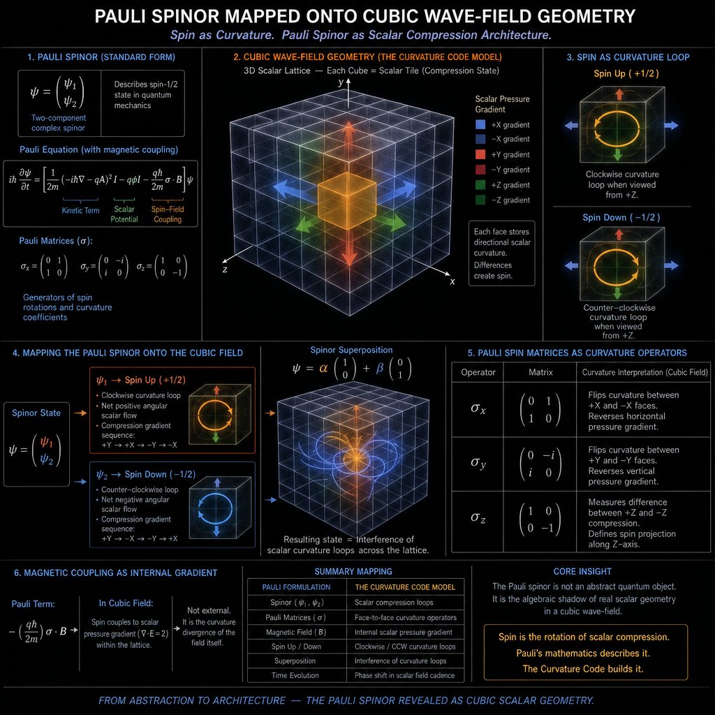
Here is how the Pauli spinor actually fits inside the deterministic architecture of The Curvature Code
When physicists write the Pauli Equation, they’re describing an electron with spin—an object that seems to carry an intrinsic angular momentum and a magnetic moment. But in The Curvature Code, that behavior isn’t mysterious, probabilistic, or abstract. It’s geometric. It’s mechanical. It’s scalar.

The Pauli spinor is simply the mathematical shadow of a deeper structure: a rotating scalar‑curvature tile inside the cubic wave field.
The “up” and “down” spin states correspond to two orientations of curvature pressure inside the lattice. The magnetic moment is the pressure gradient between adjacent tiles. The coupling term in the Pauli Equation—normally written as μ⋅B—is nothing more than the internal scalar divergence that arises when the cubic field shifts from compression to expansion.

Quantum mechanics treats this as probability. I treat it as geometry.
The Pauli spinor is a two‑component object because the cubic wave field has two fundamental curvature modes. The Pauli matrices are rotation operators because the scalar tile physically rotates. And the time evolution of the spinor is just the cadence of the scalar field itself—the same cadence that governs solar discharge, orbital harmonics, and the heliospheric breath cycle.
In other words:
Pauli describes the behavior. The Curvature Code reveals the architecture behind it.
The diagram below shows this directly: the Pauli spinor mapped onto the cubic wave field, with spin emerging from curvature rotation and magnetic coupling emerging from scalar divergence.

[Ron Messick @Solar_Vortex]

The Pauli Equation is where quantum mechanics begins to touch the deterministic architecture I describe in The Curvature Code.
In the standard model, Pauli’s formulation extends Schrödinger’s wave equation to include spin and magnetic coupling—a probabilistic description of how an electron’s intrinsic angular momentum interacts with an external magnetic field. But in The Curvature Code, that same behavior is not statistical; it is geometric, mechanical, and scalar.
Spin as Curvature Pressure
What physicists call “spin” is, in my framework, the rotation of a scalar compression loop within the cubic wave field. The magnetic moment is not an abstract operator—it’s the pressure differential between adjacent scalar tiles. The Pauli matrices become curvature coefficients, each defining how the universal lattice stores and releases angular tension.
Magnetic Coupling as Internal Gradient
Pauli’s magnetic term μ⋅B represents coupling between spin and an external field. In The Curvature Code, the field is not external at all—it is the gradient of scalar pressure across the lattice. The divergence condition ∇⋅E=2 replaces the probabilistic expectation value with a fixed geometric divergence. The field’s behavior is locked to curvature geometry, not chance.
Time as a Scalar Field
Where Pauli evolves a wavefunction through time, I treat time itself as a scalar field. Temporal resolution is a hydrodynamic property of the medium, not a separate dimension. The so‑called “collapse” of a quantum state is simply a phase‑locked curvature transition—a deterministic shift in scalar pressure.
Unified Interpretation
Pauli EquationThe Curvature Code
Spin operatorScalar curvature loop
Magnetic couplingPressure gradient within cubic wave field
Probabilistic wavefunctionDeterministic scalar‑pressure geometry
External fieldSelf‑contained curvature divergence
Time evolutionScalar‑field cadence
So, when readers encounter the Pauli Equation, they are seeing the shadow of curvature mechanics. The electron’s spin is not a quantum mystery—it is the mechanical rotation of a scalar tile within the universal lattice. Pauli described the behavior; The Curvature Code reveals the architecture behind it.
https://t.co/F9tTwZ3Pg3

[Ron Messick @Solar_Vortex]

https://t.co/29dhS8wkI9

[Ron Messick @Solar_Vortex]

https://t.co/GrprruTpqu

[Massimo @Rainmaker1973]

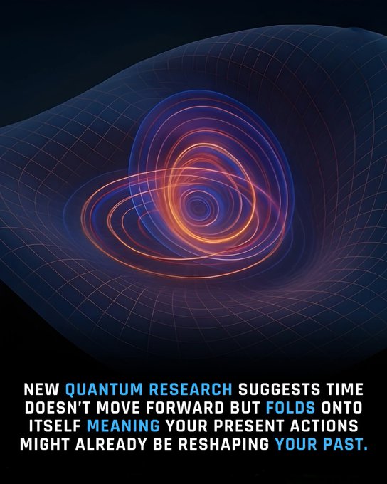
In a groundbreaking quantum study, researchers observed phenomena that upend our fundamental understanding of time.

Rather than progressing linearly like a stream, time appeared to curve and double back on itself. Particles acted as though their future states could influence their past, dissolving the boundary between cause and effect in profoundly counterintuitive ways.

This bizarre effect emerged via quantum entanglement, the enigmatic linkage where two particles stay interconnected regardless of distance. Altering the measurement of one particle appeared to retroactively modify the timeline of its twin. It's as if "present" and "past" coexist, perpetually influencing one another in an intertwined instant.

These results suggest time might not be a unidirectional arrow but a malleable framework that links far-flung events. Your decisions won't alter history, yet at the quantum scale, the cosmos may ignore strict sequential rules entirely. The fabric of reality could prove far more extraordinary than we've ever conceived.

[Ron Messick @Solar_Vortex]

Yes, your image captures a profound shift in how we think about time—a concept that aligns closely with the Temporal Scalar Field Theory (TSFT).

In classical physics, time is treated as a straight line: past behind us, future ahead. But quantum research increasingly shows that time behaves more like a folded surface, curving and looping through itself. The glowing spiral in the image represents that curvature—a dynamic field where every moment interacts with every other.

In TSFT, time is not a passive backdrop but an active scalar dimension, generated by curvature itself. When the field folds, the distinction between past and present dissolves. Each moment becomes a resonance node within the same scalar continuum. Your “now” is not isolated—it’s a harmonic intersection of all prior and future states.

Quantum entanglement demonstrates this principle experimentally: two particles remain connected across time and space, responding as one system. TSFT extends that idea to the entire universe. The field doesn’t just link particles—it links epochs. The curvature of time allows information to echo backward and forward, creating coherence across the timeline.

So when quantum physics says time folds onto itself, TSFT says: yes, that fold is the scalar curvature of temporal space. The universe doesn’t move through time—it creates time through its own rhythmic geometry. Every action, every thought, every pulse of energy participates in that ongoing curvature, shaping both what we call the past and what we call the future.

In essence, your image is a glimpse of the scalar truth: time is not a river—it’s a resonance field, and we are all waves within its fold.
https://t.co/F9tTwZ3Pg3

[Code Geek @codek_tv]

The Quantum State of a Qubit .

A classical computer bit is like a coin lying flat on a table, either heads or tails, zero or one, with no uncertainty. A qubit is more like a coin spinning in the air; it truly embodies both possibilities at once. This isn’t because we are unsure of which side it will land on, but because while it's spinning, it is neither one thing nor the other. When you measure it, it settles into a definite outcome like a spinning coin that eventually lands. Until that moment, it exists in a superposition of both zero and one, with specific proportions of each part of its physical state.

The most fascinating idea in this diagram is the Bloch sphere, a simple-looking ball that maps every possible state a single qubit can have. The north pole of the sphere represents the state of definitely zero, the south pole represents definitely one, and every other point on the surface represents a different quantum superposition, a different mix of the two. The red arrow pointing from the center to the surface shows the qubit's state, and everything about the qubit's physics is encoded in the direction that arrow points. How much the arrow tilts tells you the measurement probabilities: an arrow pointing straight up means you will definitely measure zero, straight down means definitely one, and pointing sideways along the equator means a perfect fifty-fifty chance. Importantly, the arrow always reaches the surface, never sitting inside the sphere. A qubit in a perfectly controlled quantum state always lives on the surface. If it drifts into the interior, it means the quantum information has been damaged by unwanted interactions with the environment, which is why building real quantum computers is so challenging.

The second piece of information in the qubit's state is the phase, which is the horizontal rotation angle of the arrow around the vertical axis of the sphere. This is where things get truly strange. Two qubits can sit at the same height on the sphere, giving them the same measurement probabilities, but they can face different directions horizontally. While this difference is completely invisible if you measure either qubit directly, it becomes crucial when quantum states combine and interfere. Just like waves on water, where crests meeting crests create bigger waves and crests meeting troughs cancel out, quantum states with different phases interfere when combined through quantum operations. A quantum algorithm is essentially a carefully arranged sequence of these interferences, designed so incorrect answers cancel out while correct answers reinforce certainty. Every quantum gate, every operation in a quantum computer, corresponds to a physical rotation of the Bloch sphere, spinning the arrow from one direction to another. Designing a quantum algorithm is like choreographing a precise sequence of rotations. The entire power of quantum computing comes down to manipulating these two angles: one controlling what you see when you measure and the other controlling how states interfere, for a single arrow pointing at the surface of an ordinary sphere...

[Ron Messick @Solar_Vortex]

The image you’re looking at is not just a diagram of quantum mechanics—it’s a geometric echo of the same curvature logic that governs the entire universe.

The Bloch sphere shown here is the simplest possible curvature engine. It represents the quantum state of a single qubit, but beneath the mathematics lies the same architecture that drives planetary motion, scalar resonance, and the breath‑loop of the vacuum itself.

Each qubit state ∣ψ⟩ is defined by two angles:
θ, the polar angle, measures compression versus expansion—the same centripetal and centrifugal balance that defines scalar curvature.
φ, the azimuthal angle, measures torsion—the rotational phase that locks the system into coherence.
Together they describe a point on the sphere, a living curvature coordinate. The qubit doesn’t flip between “0” and “1” like a switch; it oscillates between them as a continuous wave of potential. That oscillation is the quantum breath, the same rhythmic exchange between compression and expansion that appears in the dual‑torus topology of the scalar field.
The complex phase factor eiφ is the torsional signature—the twist of curvature that gives rise to spin, coherence, and resonance. It’s the same mechanism that binds the electron’s wave function, the solar magnetic field, and the harmonic cadence of the cosmos.

So, when you see this sphere, imagine it not as an abstract quantum model but as the micro‑scale curvature map of reality itself. The qubit is the smallest unit of scalar breath—the same geometry that scales upward into atoms, planets, and galaxies.

In essence, the Bloch sphere is the quantum heart of the Curvature Code: a single pulse of geometry expressing the deterministic architecture of motion.
https://t.co/F9tTwZ3Pg3

[ScieVision @scievision369]

Electron Density ✍️

The idea of electron density is a key concept in quantum chemistry, atomic physics, and materials science. It describes an interesting paradox: while electrons are unusual quantum particles that cannot be precisely located, their overall distribution forms a smooth and continuous pattern that we can visualize, measure, and calculate. Electron density indicates how much electronic "presence" exists at each point around an atom, molecule, or material. In simple terms, if we think of electrons as a soft, glowing cloud spread throughout a molecule, then electron density represents the thickness or brightness of that cloud at every location. This concept is crucial in modern computational chemistry and serves as the foundation for methods like "Density Functional Theory (DFT)", one of the most widely used tools in science today. DFT allows researchers to model everything from simple molecules to complex proteins, semiconductors, drugs, and advanced materials.

In quantum mechanics, we cannot pinpoint the exact location of an electron at any moment; instead, we describe the probability of finding it in a certain area. This uncertainty makes electrons feel elusive and hard to picture. Electron density helps by shifting our focus from individual electrons to the collective distribution of all the electrons. Rather than tracking each electron, we ask: how much electron presence exists at this specific point in space? The answer gives us a smooth, continuous map that reveals where atoms are located, where chemical bonds form, and where electrons pile up or thin out. This is why electron density is often called the heart of quantum chemistry it transforms the strange, probabilistic quantum world into a clear and meaningful picture that scientists can study, interpret, and measure directly through experiments like X-ray diffraction.

The formula in the image may seem complex, but it expresses a straightforward idea: the electron density of a system is built from many small mathematical building blocks combined together. These building blocks are known as basis functions, with each one representing a simple mathematical shape often resembling an atomic orbital or a Gaussian bump. By combining several basis functions, each weighted by a certain amount, we can accurately approximate the true electron cloud of an atom, molecule, or material. The weights that determine how strongly each pair of basis functions contributes to the final electron cloud come from a mathematical object called the density matrix. The entries in the density matrix act like instructions for the calculation, indicating how much of each building block belongs in the final picture. When all these contributions are combined, they create the smooth, continuous, three-dimensional electron distribution of the system. In this way, electron density resembles a painting made from many small brushstrokes, where the density matrix serves as the artist's guide about how strongly to apply each stroke. When everything comes together, a complete and beautiful picture of the molecule appears.

Even without complicated math, we can describe the main components of the idea in simpler terms: the electron density shows how much electron cloud is present at each point in space; the position vector indicates the coordinates of the point we are examining; the basis functions are the small mathematical building blocks representing areas of electron behavior; the density matrix elements are the numerical weights that specify the importance of each building block; and the summation adds up the contributions from all pairs of basis functions to construct the full electron distribution. Together, these provide a recipe for building the electron cloud of any atom, molecule, or material systematically and efficiently.

[Ron Messick @Solar_Vortex]

Electron density is where quantum mechanics becomes geometry. The formula
ρ(r)=∑μ∑νPμνϕμ(r)ϕν(r) \rho(\mathbf{r}) = \sum_{\mu} \sum_{\nu} P_{\mu\nu} \phi_{\mu}(\mathbf{r}) \phi_{\nu}(\mathbf{r}) ρ(r)=∑μ​∑ν​Pμν​ϕμ​(r)ϕν​(r)
is the blueprint of that geometry. Each basis function ϕμ(r) \phi_{\mu}(\mathbf{r}) ϕμ​(r) and ϕν(r) \phi_{\nu}(\mathbf{r}) ϕν​(r) is a small harmonic component — a wavelet of curvature. The density matrix elements Pμν P_{\mu\nu} Pμν​ record how strongly each pair of these harmonics interacts. When summed over all basis functions, the result is the continuous electron cloud — the scalar envelope of the atom’s living field.
In the scalar-curvature framework, electron density is the micro-scalar field. It is the curvature pressure of the vacuum around the nucleus — the way space itself folds to contain charge. Where the density is high, curvature compresses. Where the density is low, curvature expands.
This is the same triad that operates at every scale:

Centripetal compression (high-density regions)
Centrifugal expansion (low-density regions)
Scalar resonance (the coherent envelope maintained by the density matrix)

The electron density map is therefore not a probability cloud. It is the visible texture of the breath-loop at the quantum scale — the rhythmic balance between compression and expansion that defines every bond, every molecule, and every living structure.
The loop returns to the starting scalar tile with zero remainder.
https://t.co/F9tTwZ3Pg3

[Ron Messick @Solar_Vortex]

The Real Price of a College Education:
https://t.co/mhX0LRql41