Anthony Bardou

Postdoctoral Researcher @EPFL. Bayesian / Black-Box Optimization and their applications. Prev. @ENSdeLyon

[CNRS Sciences informatiques @CNRSinformatics]

#Distinction 🏆| Le @GdrRsd a récompensé trois chercheurs et chercheuse pour leurs travaux de thèse. Il distingue des contributions dans des domaines variés sur l’optimisation.
➡️ https://t.co/9qs3Ept01X
🤝 @LIGLab @CnrsAlpes @CNRS_dr07

[Anthony Bardou @abardou_]

cc @EPFL @NeurIPSConf #BayesianOptimization

[Anthony Bardou @abardou_]

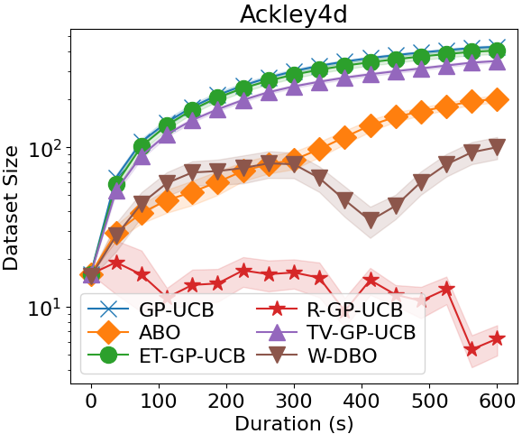
Clearly, W-DBO achieves a much lower average regret, because it is the only one able to explore the hole at the center of the domain. All the other average regrets skyrocket at the middle of the experiment, because they miss that hole.

[Anthony Bardou @abardou_]

That's the end of the thread! If you want to deep dive in the paper, here are a couple of links for you.

arXiv: https://t.co/xRCHMcg3zz
GitHub: https://t.co/QB3vLT3341

Naturally, you can also come find me at NeurIPS, I'll be happy to have a chat about it!

[Anthony Bardou @abardou_]

We consider the 4-dimensional Ackley function. One of the dimensions is the temporal one, the others constitute the parameters space.

And here is the average regret and the dataset size of W-DBO compared to the state-of-the-art on this benchmark.

[Anthony Bardou @abardou_]

A noisy black-box is a stingy function. Given an input x, it will only yield y(x) = f(x) + ε, ε ~ N(0, σ²). There is no way to get higher-order information (e.g., ∇f(x)).

Optimizing a noisy black-box is hard. Optimizing a dynamic black-box is much harder, for three reasons⬇️

[Anthony Bardou @abardou_]

How does W-DBO perform in the benchmarks then?

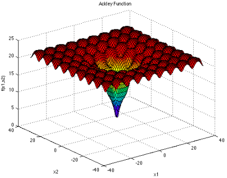
Let me illustrate its performance with one of the synthetic benchmarks we considered. Here comes the Ackley function!

It has an almost flat region full of local minima on the outer part of the domain, and a deep hole at its center.

[Anthony Bardou @abardou_]

WD combines these two types of relevancy in a principled way, as can be seen in the visualization.

Clearly, a lot of redundant observations get rapidly deleted. As an interesting consequence, the resulting dataset is not simply made up of the last n observations.

[Anthony Bardou @abardou_]

Using the WD as a measure of relevancy brings an additional perk: it accounts for both temporal relevancy (staleness) and spatial relevancy. In fact, if two queries are close in the spatial domain, then one of them is likely to get deleted for not being informative enough.

[Anthony Bardou @abardou_]

And that's where the Wasserstein distance (WD) meets Bayesian optimization🤝🏼We use the WD between our two posteriors GP(D) and GP(D') as a measure of relevancy.

Using it, our algorithm, W-DBO, defines a policy to remove stale observations in an online, more refined fashion.

[Anthony Bardou @abardou_]

Formally, consider a GP surrogate conditioned on the entire dataset of observations D = {((xk, tk), yk)}, 1 <= k <= n, and denote it GP(D).

Now, consider D' = D \ {((xi, ti), yi)} and GP(D').

If the i-th observation is irrelevant, GP(D) and GP(D') should be similar.

[Anthony Bardou @abardou_]

Before going further, let us define what I mean by an irrelevant observation.

Here's an intuitive definition: an observation is irrelevant if removing it from the dataset has little effect on the prediction made by our surrogate model, usually a Gaussian process (GP).

[Anthony Bardou @abardou_]

DBO algorithms in the literature either completely ignore this problem (i.e., do not remove stale data) or address it with a very drastic procedure: they periodically reset their datasets, probably deleting a lot of relevant observations in the process.

[Anthony Bardou @abardou_]

Reasons (2) and (3) are bad news. A dynamic BO (DBO) algorithm cannot endlessly accumulate stale data in its dataset without hampering its sampling frequency.

Consequence: it has to pinpoint stale observations, and remove them in an online fashion!

[Anthony Bardou @abardou_]

(3) Sampling frequency. This one is a direct consequence of (2). Because each observation eventually becomes stale, the BO algorithm has to sample the black-box frequently enough so that its dataset does not become entirely irrelevant to make predictions about f.

[Anthony Bardou @abardou_]

(2) Stale data. Unlike the static black-box optimization problem, an observation ((x, t), y(x, t)) may become irrelevant for predicting how the dynamic black-box will behave in the future. At this stage, it becomes a computational burden for the BO algorithm.

[Anthony Bardou @abardou_]

(1) No time travel. At time t, only f(•, t) is observable. Any f(•, t'), where t' < t, belongs to the past and is no longer observable. Any f(•, t') belongs to the future and is not observable yet.

[Anthony Bardou @abardou_]

Struggling with the optimization of a dynamic black-box function?

Our latest research introduces a game-changer for dynamic Bayesian optimization and will be presented at NeurIPS'24 next December!

As we await the lively poster chats, here's a sneak preview of how it works🧵⬇️