AI with Alex

AI, vibe coding, software, and share knowledge whatever’s on my mind.

[AI with Alex @alexbloomberg_]

@faultbugs

[AI with Alex @alexbloomberg_]

The overall process of Fine-tuning a InstructModel: #LLM #LLMs

[AI with Alex @alexbloomberg_]

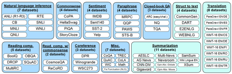
The performance gains brought by instruction tuning exhibit a pronounced large-model effect.

It turns out only when the model scale reaches around tens of billions of parameters(68B–137B) does instruction tuning bring improvements on out-of-distribution tasks. #ScalingLaw #FLAN

[AI with Alex @alexbloomberg_]

FLAN Instruction Tuning:
Using instruction tuning to improve the model's zero-shot capabilities

The 62 natural language processing tasks are divided into 12 categories.

For each task, 10 unique instruction templates are manually constructed.

[AI with Alex @alexbloomberg_]

Attackers can run malicious code on vulnerable systems without logging in. Users should immediately prepare for installing patches for affected assets; If the repair patch cannot be installed, consider taking the affected website offline or restricting or isolating from out.#php

[国家サイバー統括室(注意・警戒情報) @cyber_forecast]

PHPのセキュリティチームが、重大な２件の脆弱性に関する注意喚起を行っています。公開しているウェブサイトでPHPを使用しているか確認し、10月21日午後11時（日本時間）に公開される修正パッチについて、可及的速やかに適用できるよう準備をお願いいたします。
https://t.co/TFPc8QIdUN

[AI with Alex @alexbloomberg_]

K-Means Clustering

#MachineLearning #Python #KMeans #ScikitLearn #DataScience #LLM

[AI with Alex @alexbloomberg_]

Word ID → Search embedding matrix → Obtain word vector
→ Enter each layer of Transformer
→ Output prediction
→ Calculate Entropy loss
→ Backpropagation
→ Update embedding matrix #LLM

[AI with Alex @alexbloomberg_]

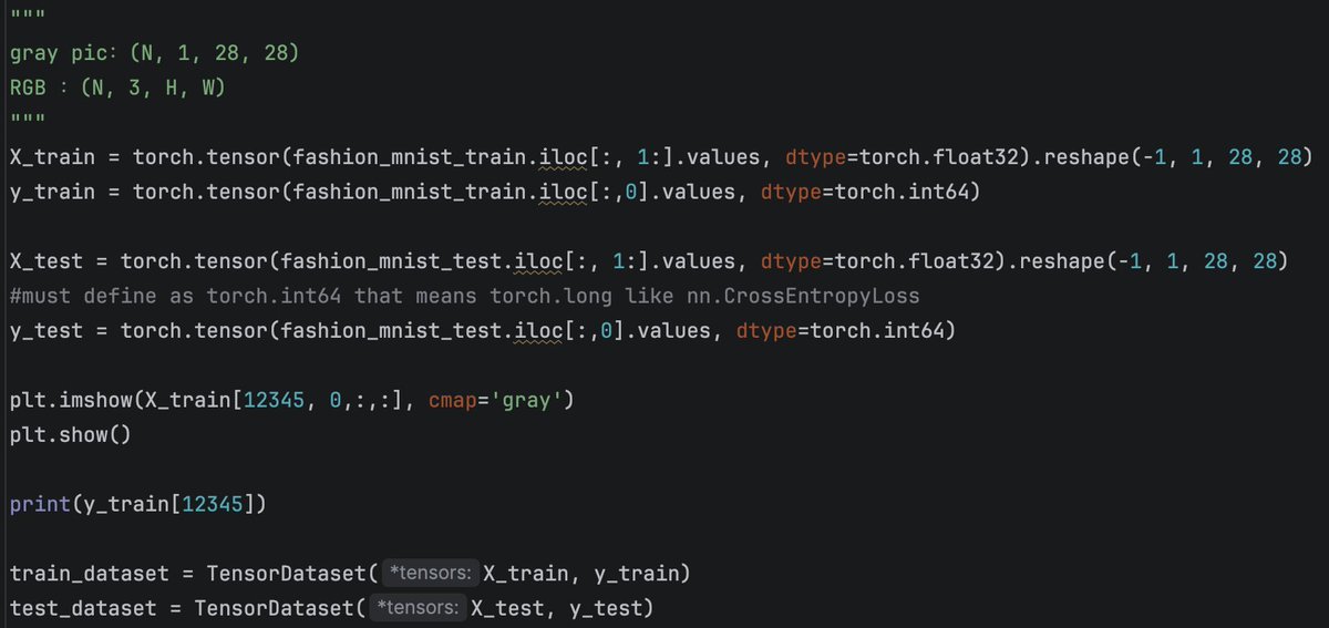
OH = (H+2P-FH)/S + 1;OW: same calculate as OH.If the input shape is (N, 1, 28, 28) and conv layer is nn.conv(in_channels:1, out_channels:6, kernal_size:?, stride:1, padding:2), we can reverse deduce the shape of kernal_size to be (5, 5). #Python #LLM

[AI with Alex @alexbloomberg_]

Similar in Transformer:

for y=x+Attention(x)

The responsibility is not recreating a new complete x, but rather, based on the current x, what information do I think should be supplemented or modified. That's why Transformers can stack dozens or even hundreds of layers. #LLM

[AI with Alex @alexbloomberg_]

H (x) ≈ 0, so y ≈ x; If changes are needed, learn the corresponding H (x). At the same time, Shortcut provides the "1" in ∂ y/∂ x=1+∂ H (x)/∂ x, allowing gradients to propagate directly, thereby alleviating the problem of gradient vanishing in deep networks. #LLM #GPT

[AI with Alex @alexbloomberg_]

The core of ResNet is to divide the input x into two paths through residual connections: one path directly retains the original information through shortcut, and the other path learns the information that needs to be supplemented or modified on x through layer learning to obtain

[AI with Alex @alexbloomberg_]

H (x), and finally outputs y=x+H (x). The network does not know in advance whether it needs to be modified or not, but learns it through training loss → backpropagation → parameter updates: if the current block does not need to change information, it will gradually learn that

[AI with Alex @alexbloomberg_]

Adam: Fast and steady, take the shortcut directly

Note that they are optimized using different learning rates.

#DeepLearning #MachineLearning #PyTorch #AI #Optimization

[AI with Alex @alexbloomberg_]

The same "canyon", four ways to traverse 🏔️

SGD: Jump left and right, moving like a sawtooth

Momentum: Incorporating inertia makes it much smoother

AdaGrad: Strong in the early stage, but getting weaker and weaker in the later stage

[AI with Alex @alexbloomberg_]

Determine if it has ended?
- Yes → Output Final Answer
- No → Return to the planning stage and enter the next round #LLM

[AI with Alex @alexbloomberg_]

Input query
↓
Cumulative context (all historical plans+execution results)
↓
[ Planning Stage ] Planner
↓
Generate<Plan_i>, which contains multiple independent<prompt_i. j>subtasks internally
↓
[Parallel Execution Stage] Executor Pool
↓

[AI with Alex @alexbloomberg_]

Assign an executor to each<prompt_i. j>and generate inference results in parallel
↓
[Synchronization Phase] Sync
↓
All execution results are packed back into cumulative context in order
↓

[AI with Alex @alexbloomberg_]

After training, W is frozen for inference. It is not "set once after one backpropagation" nor "finding the global minimum", but rather iterative optimization until convergence. #LLM #GPT

[AI with Alex @alexbloomberg_]

The W of LLM is initially randomly initialized according to a specific strategy, and during training, it is repeatedly updated through backpropagation to calculate gradients + optimizer to make the Loss converge to a lower value.

[AI with Alex @alexbloomberg_]

If you are using PyTorch with MPS to accelerate model training on the Mac GPU, use below:
```
device = torch.device( "mps" if https://t.co/fMlOZvE2lh_available() else "cpu")
```
#PyTorch #LLM #NP