qewrd

no

[リニア・テック 別府 伸耕 @linear_tec]

「熱力学」の原稿を書いています．

ガソリン・エンジンをモデル化した「オットー・サイクル」のアニメーション．
https://t.co/IGVPQMrIQk

[Harley Anime✨ @dbs_10_10]

Goku meets Grandpa Gohan😭✨

[PlayStation Park @PlayStationPark]

'Metal Gear Solid'
PlayStation

[Matheorems @matheorems]

In the static regime, the electric and magnetic fields generated by point sources are the superposition of radial monopoles and dipoles.

Electric field:
∑ qᵢ (x − xᵢ) / ‖x − xᵢ‖³
Magnetic field:
∑ [3 rᵢ ⟨rᵢ, m⟩ − m] / ‖x − xᵢ‖³

where rᵢ = (x − xᵢ) / ‖x − xᵢ‖

[ScieVision @scievision369]

Laurent Series ✍️

Here is something that should feel deeply unsettling. Mathematics has a tool called the Taylor series that can represent almost any well-behaved function as an infinite sum of terms, and it works beautifully almost everywhere. But at certain special points, called singularities, functions blow up to infinity, become undefined, or behave irregularly. At these points, the Taylor series completely collapses. It cannot be constructed there. It gives no information. It simply fails.

What makes this unsettling is that those singular points, where the standard tool breaks down, are often the most interesting and important points in the entire function. In quantum mechanics, singularities correspond to actual particles and resonances. In fluid dynamics, they correspond to vortices and flow sources. In electrical engineering, they correspond to the natural frequencies of circuits. The mathematical tool fails exactly where you most need it to work.

Pierre Alphonse Laurent, a French military engineer from the 1840s, refused to accept this failure. He wondered what would happen if you extended the Taylor series in a natural but previously unexplored direction. What if, instead of only allowing positive powers of the variable, you also allowed negative powers? What if the infinite sum ran not just forward toward higher positive powers but also backward toward more negative powers? The answer to that question is the Laurent series, and it transforms singularities from obstacles into readable mathematical objects.

To understand why negative powers matter so much, think about what they do near a singularity. When you raise something to a positive power and let it approach zero, the result also approaches zero. Positive power terms vanish near the singular point and cannot capture explosive behavior. But when you divide by something, which is what a negative power means, and let the denominator approach zero, the result blows up to infinity. Negative power terms naturally grow without bound near singularities, which is exactly the behavior that needs to be captured and described. By including them in the series, Laurent gave mathematics the vocabulary to express singular behavior instead of falling silent in its presence.

The geometry of where Laurent series work is also beautiful and worth appreciating. Taylor series work inside circular discs points within a certain radius of the center. Laurent series work in annular regions ring-shaped areas between two concentric circles, like the cross-section of a hollow tube. The inner circle of this ring excludes the singularity itself, keeping it at a safe distance. The outer circle marks the boundary beyond which the next singularity disrupts the series. The ring-shaped region between them is where the Laurent series lives and works perfectly. In the diagram, this ring is the green shaded area between the blue inner circle and the red outer circle, with the winding curve gamma tracing a path inside this ring, always staying between the two boundaries.

Now here is the most exciting part: what the Laurent series reveals about singularities. By examining how many negative power terms appear in the series with non-zero coefficients, you can immediately read the precise character of the singularity, classifying it into one of three distinct types.

If there are no negative power terms, the singularity is what mathematicians call removable. The function only looks singular because of how its formula is written the apparent breakdown is an illusion. The Laurent series reveals that the function is actually smooth and well-behaved near that point, and you can eliminate the singularity entirely by defining the function's value properly there. The singularity was never real; it was a mathematical mirage.

[Mathematica @mathemetica]

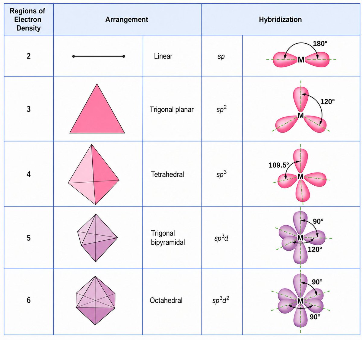
Electron density regions around a central atom set the molecular arrangement through orbital hybridization.

- Two regions produce a linear form with sp hybrids at 180°.
- Three give trigonal planar geometry via sp² hybrids at 120°.
- Four create tetrahedral structures using sp³ hybrids at 109.5°.
- Five form trigonal bipyramidal shapes with sp³d hybrids at 90° and 120°.
- Six yield octahedral arrangements through sp³d² hybrids at 90°.

Octahedral sp³d² hybridization is applied by materials scientists in transition-metal complexes to engineer ligands for industrial hydrogenation catalysts that convert alkenes into saturated hydrocarbons.

[naruto13 @Dylangig]

Minuto 70, Inglaterra ganando 1-0

Molina 🔄 Montiel

[Peñargrol @CAPArgento__]

"ayy como vas a gritar un gol de congo"

yo en el living de mi casa:

[ScieVision @scievision369]

Lyapunov Stability Theory ✍️

It is an easy way to see if a system will settle down at its balanced resting point. Think of the resting point as the bottom of a bowl. You set up a specific "height" measurement that is zero only at the bottom and higher everywhere else. If this height always goes down as the system moves, like a ball rolling downhill, then no matter where you start nearby, the system will slide down and stay at the bottom forever. The red spiral path in the picture shows this happening. This shows the system is stable and will return to balance after small disturbances, without needing to solve complicated math.

[Pink Floyd 💎 @Just_pinkfloyd]

In The Flesh

[silly reigen bot @sillyreigenbot]

happy new year !

[Nostalgia @nostalgiaa]

Monster

[Vicente Viloni @_VicenteViloni]

HOY AMANECÍ EN SILENT HILL 🤯

[La Hora Del Metal @horametalradio]

Así estoy.

[Old Internet @OldInternetFeel]

CERN, 2004