Kyle Walker

Professor and entrepreneur working on topics in geospatial, AI, and open source software.

Building AI solutions for energy:

[Kyle Walker @kyle_e_walker]

@qvant_ haha appreciate it! love NBA Jam

[Kyle Walker @kyle_e_walker]

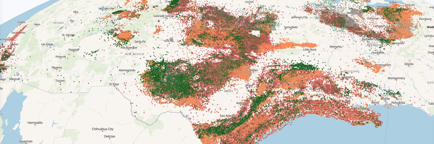
Texas operators injected 7.77 billion barrels of oilfield wastewater into saltwater disposal wells in 2024, up from 4.37 billion in 2015.

Cataloged earthquakes of magnitude 2.5 and up in Texas went from 60 in 2015 to a peak of 816 in 2022.

Explore both on today's map.

I added something I've never done on a map before: actual sound. Use the play button to animate earthquakes, and each earthquake plays a timpani sound as it happens, lower and louder for bigger ones.

With headphones, West Texas earthquakes will be louder in your left ear, and East Texas louder in your right. (Seriously, try it).

The map plays 2015–2025 month by month, with disposal wells sized by barrels per day. The two largest earthquakes, both M5.4, hit Reeves County in November 2022 and Culberson County in May 2025.

Day 11 of #30DayMapChallenge: Sound.

Explore the map and turn the sound on: https://t.co/ZViN3TfCXH

[Kyle Walker @kyle_e_walker]

@Cash_Cameron thanks! was fun to see what Fable can do

[Kyle Walker @kyle_e_walker]

Day 10 of #30DayMapChallenge: Prompting only

I asked the brand-new Fable 5.2 to map the PNNL data centers dataset with only mapgl and R code - no custom JavaScript allowed. The prompt:

"Create the most ambitious map you can possibly make from the data center dataset, using ONLY R. You can't add custom JavaScript to the map. You have to use mapgl exclusively, or figure out a way to create the best and most impressive map you can possibly make, relying only on R code and pushing mapgl as far as you can take it."

It aggregated data centers by hexbin, then mapped them on a @Mapbox map as stacked 3D hexagonal "towers" by operator when zoomed out - a technique I'd never done before in mapgl! As you zoom in, you'll see the hexagons give way to 3D building footprints.

The map also uses mapgl's slider control to allow you to flip through views of the different operators, and uses URL hashes to allow jumping to different views, as those actions are Shiny-only in mapgl - which gets around the no custom JavaScript restriction.

You can find the map, along with all of this month's maps, at https://t.co/tIN1OtkYBZ.

The R code (both data wrangling and mapping) is downloadable from the map if you want to try it out and see how Fable came up with these techniques.

[Kyle Walker @kyle_e_walker]

For Day 9 of #30DayMapChallenge: Urban/Rural, we're celebrating the release of the 2024 LODES dataset from @uscensusbureau.

LODES gets you block-level data on workplace, residence, and origin-destination flows for the US workforce. It's one of my all-time favorite datasets.

For the map challenge, I've updated my LODES WAC dot map for 2024, mapping 153 million jobs across all of the US's urban and rural areas. AK and MI are back-filled to the most recent year available.

There's also a cool new feature in mapgl which now ships with interactive categorical legends. Long-click (or long-press) a legend entry to isolate it, which makes it a lot easier to explore individual categories.

All of this month's maps are here: https://t.co/tIN1OtkYBZ

[Kyle Walker @kyle_e_walker]

Day 8 of #30DayMapChallenge: Utopia.

I've mapped a "utopian" scenario for the Texas grid, where every project waiting to connect actually gets built.

On the left: ERCOT's power plants and batteries today, 182.6 GW of generating and storage capacity.

On the right: the same grid plus the 1,680 publicly listed projects in ERCOT's interconnection queue. That comes to about 616 GW, roughly 3.4x what's there today. Most of it is solar and batteries.

Drag the slider to compare the two. I've put a methodology note on the map as well (as matching the interconnection queue to geographies is inexact).

All of this month's maps are here: https://t.co/SgKtYHkk1H

[Kyle Walker @kyle_e_walker]

@dfrodriguezl @Mapbox I did the quick and dirty version for the map challenge, block groups based on their population-weighted centroids (which are now in tigris, by the way!)

[Kyle Walker @kyle_e_walker]

Day 7 #30DayMapChallenge (10 minute map).

About 58% of Texans, an estimated 17.4 million, live within a 10-minute drive from a public DC fast charger.

Click anywhere or search a for your city to see your 10 minute coverage.

Basemap and isochrones from @Mapbox.

Browse all of this month's maps on energy and infrastructure here: https://t.co/tIN1OtkYBZ

[Kyle Walker @kyle_e_walker]

@mepa1363 didn't have to do much, they were already georeferenced! I just clipped them to their neatlines first

[Kyle Walker @kyle_e_walker]

Day 6 of #30DayMapChallenge: Vintage.

The Permian Basin in the 1950s and today.

On the left: four 1957–58 Army Map Service topographic sheets, which mark wells as small circles along with oil fields, pipelines and tanks.

On the right: satellite imagery of the same area with the 447,665 wells on record today.

The map opens on the Kermit and Wink oil fields in Winkler County. Drag the slider to compare the two map views.

Georeferenced maps are from USGS's Historical Topographic Map Collection, uploaded to @Mapbox and served as raster tiles.

All of this month's maps are here: https://t.co/SgKtYHkk1H

[Kyle Walker @kyle_e_walker]

@AzizSunderji Love LODES. We got 2024 data yesterday, did you see?

[Kyle Walker @kyle_e_walker]

The 447,665 wells on this map come from the Texas and New Mexico well data I compile at Clearfork Intelligence.

If you research wells in the Permian, Wells Intelligence lets you filter wells, select them with a lasso on the map, and compare production histories:

https://t.co/S9BqtMOSMk

[Kyle Walker @kyle_e_walker]

@NiyerEnergy this was my favorite one so far. tomorrow's is good too!

[Kyle Walker @kyle_e_walker]

In @Mapbox GL JS, you've been able to add custom 3D models as model layers for a while.

The hard part has always been making the glTF models.

With Claude Opus 5.5 and Blender, those of us without 3D modeling expertise can now build models ready for mapping.

A great use case is showing proposed or in-progress construction, like Saudi Arabia's Jeddah Tower, which is set to become the world's tallest building.

In R's mapgl, I've just added support for these models. Use add_model() and add_model_layer() to put a model at the right spot on your map, customize its look, cast shadows, and more.

It's in the development version on GitHub: pak::pak("walkerke/mapgl")

[Kyle Walker @kyle_e_walker]

The new Opportunity Zone 2.0 designations have been released!

Copy-paste this into R to start exploring:

library(readxl)
library(tigris)
library(dplyr)
library(mapgl)

us_tracts <- tracts(cb = TRUE)

oz_url <- "https://t.co/6wxY9Ti1xf"
oz_file <- "oz.xlsx"

download.file(oz_url, destfile = oz_file, mode = "wb")

oz <- read_excel(oz_file)

oz_geo <- filter(us_tracts, GEOID %in% oz$`Census Tract Number`)

maplibre_view(oz_geo)

[Kyle Walker @kyle_e_walker]

@milos_gis yeah this one was really interesting! I've been thinking about this sort of analysis for a while

[Kyle Walker @kyle_e_walker]

For Day 5 of #30DayMapChallenge: Sight, I've done a viewshed analysis for wind turbines in Nolan and Taylor counties in Texas and mapped it with Mapbox.

This one was a really interesting research project leading to some new features in mapgl.

On the map, the colors show how many turbine blade tips are in line of sight from each spot on the ground, out to 25 miles.

Zoom in and the turbines appear as 3D models, built in Blender and scaled to their real size, using new 3D model support in R's mapgl package.

Viewshed rasters were pre-computed in R with terra and pulled in on turbine click. Estimated visibility comes from Argonne National Laboratory field research on how far away wind facilities stand out.

The observer is the blade tip, the target is a person's eye about 5.6 feet above the ground, and the calculation corrects for Earth's curvature and atmospheric refraction. Elevation comes from USGS 3DEP.

All of this month's maps are here: https://t.co/SgKtYHkk1H. Give this one a look and definitely try making your own 3D models and mapping them with mapgl.

[Kyle Walker @kyle_e_walker]

OpenClaw is absolutely outstanding. I run my business through it. Bots live on a secure VPS, and I interact with them (and they interact with each other) as Slack apps.

But I didn't figure out the right way to use it for nine months, and it took a couple solid days of work (with Opus 5.5 orchestrating) to set everything up the way I wanted.

So I see your point - I think people who expect this stuff to "just work" with no effort will be disappointed, but on the other hand they are revolutionary if you're willing to put the time in

[Kyle Walker @kyle_e_walker]

Day 4 of #30DayMapChallenge: Clusters.

14,797 operating US power plants from EIA data mapped as donut clusters with @Mapbox and R's mapgl package. The ring segments show capacity by fuel type.

Lots of insights in the map / data, some highlights -

About half of US power plants are solar but they make up only 12% of capacity. In contrast, gas is 13% of plants but 41% of capacity.

Texas leads in battery storage with 19.4 GW; California comes in second with 16.5 GW.

All of this month's maps, which focus on mapping energy & infrastructure, are found here: https://t.co/tIN1OtkYBZ

[Kyle Walker @kyle_e_walker]

Mapping 6,611 US solar farms for Day 3 of #30DayMapChallenge: Polygons.

Individual farms are too small to view at full national zoom, so this is a great opportunity to use "fade-on-zoom", my favorite mapping technique.

We start with hexagons colored by total solar capacity when zoomed out, fading to individual farms as you zoom in.

Zoom in even further and the polygon fill gives way to the satellite image of the solar farm itself.

Data: USGS Large-Scale Solar Photovoltaic Database https://t.co/qgEfDCh6mT

View all of this month's maps here: https://t.co/tIN1OtkYBZ