Sean Chien

PhD student in Texas A&M / Evolutionary biology

[Jen-Pan Huang 黃仁磐 @airbugshuang]

New collaboration published. Cool beetles, sky islands, local adaptation, proposing actionable plans for conservation, and more. Check it out
https://t.co/Fse4yHP4fm

[Sean Chien @Sean_Chien4]

Complete mitochondrial genome. Using long-read sequencing, we resolved the full mitochondrial genome, including the control region.

[Sean Chien @Sean_Chien4]

I’m excited to share that we’ve successfully assembled the genome of the Formosan long-armed beetle (Cheirotonus formosanus) to chromosome level with both high contiguity and completeness.
@Ecol_Evol
https://t.co/QgIEqrH4Bx

[Sean Chien @Sean_Chien4]

Sex chromosome identification. We identified both the X and Y chromosomes. Assembling the Y chromosome is challenging due to its highly repetitive content. Using a quotient approach, we successfully characterized it and even found KDM5D, a gene known to be Y-linked in mammals.

[DNLt @dnltbing]

When islands collide: Divergence predicts outcomes of secondary contact during the fusion of Sulawesi’s paleo-archipelago
[Karin et al 2025]

https://t.co/BM0Kymcmjn

[Dr. Catharine Young @DrCatharineY]

Science is not a contest to be won.
It’s a collective pursuit of truth that evolves with evidence - not a debate settled by opinion or the loudest voice.

[@EcoEvoRxiv @ecoevorxiv]

"Genomic insights into the origin of ecotypes" https://t.co/8zPfp9CKgV

[Sean Chien @Sean_Chien4]

https://t.co/rVLY7GoGEw

[National Baseball Hall of Fame and Museum ⚾ @baseballhall]

Welcome to baseball immortality, Ichiro Suzuki.

[bioRxiv Neuroscience @biorxiv_neursci]

Astrocyte Store-Released Calcium Modulates Visual Cortex Synapse Development and Circuit Function. https://t.co/YB6UvkfRVq #biorxiv_neursci

[Jen-Pan Huang 黃仁磐 @airbugshuang]

https://t.co/CLK0yTlJVf

If you’re looking for an empirical example showing the essential role of reference genomes in biodiversity conservation, here is one for you!

Our third and probably the final chapter of Taiwanese sky island stag beetle evol and con genetic is published

[Neuroscience News @NeuroscienceNew]

Brain Taps Lipid Stores for Energy During Activity

Contrary to long-held assumptions, neurons can break down fat for energy when glucose is in short supply.

In a new study, researchers found that lipid droplets inside neurons are activated by synaptic electrical activity and metabolized into fatty acids that fuel mitochondria.

This fat-burning process is controlled by the brain's activity level—more active neurons burn more fat.

Disrupting the pathway that transports fatty acids into mitochondria led to a torpor-like state in mice, highlighting its biological importance.

The findings challenge the view that fat metabolism is irrelevant to brain function.

They also suggest new avenues for understanding neurodegenerative diseases that involve disrupted energy metabolism.

[Joachim Schork @JoachimSchork]

Bayesian logistic regression is a powerful method for predicting binary outcomes (such as yes/no decisions). It differs from traditional logistic regression by incorporating prior beliefs and quantifying uncertainty using posterior distributions. This makes Bayesian logistic regression ideal for situations where you want to explicitly account for uncertainty or include prior knowledge.

Here’s a breakdown of the four key graphs that provide insights into a Bayesian logistic regression model:

✔️ Posterior Distribution Plot: This plot displays the posterior distributions of the coefficients for predictor1 and predictor2. The shaded area shows the range of probable values (credible intervals), while the vertical line marks the median estimate of each coefficient. Unlike frequentist approaches that provide single point estimates, Bayesian logistic regression gives a distribution of possible values, which allows for a clearer understanding of uncertainty in the model parameters.

✔️ Trace Plot: This shows the trace of the MCMC (Markov Chain Monte Carlo) sampling process over 4000 iterations for predictor1 and predictor2. The traces should ideally look "fuzzy" and well-mixed, moving around the full parameter space without getting stuck. This indicates that the chains have converged and that the model’s parameter estimates are reliable. A poorly mixing chain (one that looks like a straight line or is stuck) would indicate convergence issues.

✔️ Posterior Predictive Check: This plot helps to evaluate the model's predictive performance by comparing the predicted outcomes (y_rep, light blue) with the observed data (y, dark blue). The closer the predicted values align with the observed data, the better the model captures the underlying structure. In this case, the predicted values align well with the observed data, indicating a good fit. This check is crucial for assessing whether the model generates realistic predictions.

✔️ Posterior Interval Plot: This plot visualizes the credible intervals for the model coefficients, including the intercept. The wider the credible interval, the more uncertainty there is in that coefficient estimate. Both 50% (inner) and 95% (outer) credible intervals are shown, providing a range of probable values for each coefficient. If a credible interval includes zero, it means the predictor may not have a strong effect on the target variable.

This grid of graphs allows for a comprehensive understanding of your Bayesian model, showing how well the model fits the data and how much uncertainty there is in the parameter estimates. Bayesian logistic regression provides a richer interpretation than traditional methods by quantifying uncertainty and incorporating prior knowledge into the analysis.

Want more insights on data science? Subscribe to my free email newsletter!

Learn more: https://t.co/X93SeCe0rb

#datastructure #statisticians #DataAnalytics #RStats #VisualAnalytics #datavis #database

[Jim Shaw @jim_elevator]

Announcing myloasm, a new long-read (ONT R10/PacBio) metagenome assembler. With @lh3lh3.

https://t.co/ingqEXblza

[Prosanta Chakrabarty @PREAUX_FISH]

More details coming soon, but mark your calendars ...

Breakout meeting for @systbiol The Society of Systematic Biologists - will be Jan 9-11, 2026 in Baton Rouge!

Topic is 'The Importance of Natural History Collections'

@jembrown is primary organizer

https://t.co/0ZjHhXA9wu

[Rob Waterhouse also @rmwaterhouse.bsky.social @rmwaterhouse]

The ERGA BioGenome Analysis & Applications Seminar, Today, April 29th at 11:00 AM CEST, on "Genomic Erosion and Biodiversity Conservation" https://t.co/ergfO4TXyw live on YouTube! #biodiversity #genomics

[@EcoEvoRxiv @ecoevorxiv]

"The molecular evolutionary basis of species formation revisited" - https://t.co/KNSUGCpYUL

[NASA @NASA]

If you prefer to watch long-form content on YouTube, we've got you covered. Our newest documentary is available on demand. https://t.co/tOw4ebQUc5

[Joachim Schork @JoachimSchork]

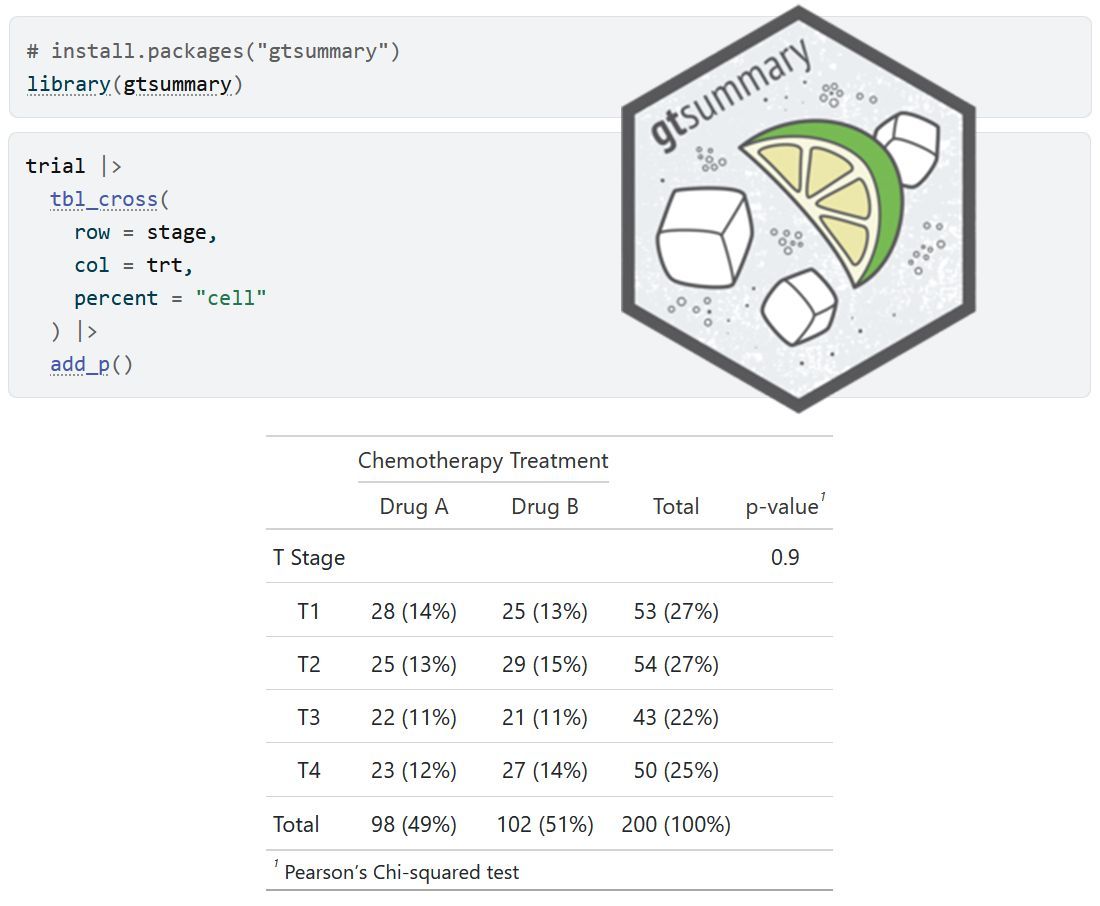
The gtsummary package in R makes it easy to create clean, publication-ready summary tables for your data. The tbl_summary() function takes a data set and generates well-organized tables that display key statistics like counts, percentages, means, and medians, which is perfect for presenting descriptive statistics in reports, manuscripts, or presentations.

✔️ Streamlines Descriptive Statistics: Quickly generates clear and professional summary tables.
✔️ Customizable: Offers flexible options for labels, decimal places, and formatting.
✔️ Supports Various Data Types: Works with continuous, categorical, and dichotomous variables seamlessly.

The visualization below shows a sample table created with tbl_summary(), illustrating its ability to organize and present descriptive statistics effectively. Visualization adapted from the official package website: https://t.co/eGJjBEUVeT

Want to explore more practical tips on Statistics, Data Science, R, and Python? Subscribe to my email newsletter!

Learn more: https://t.co/X93SeCe0rb

#RStats #datastructure #coding #DataScience #Rpackage