Oscar Cortes

[Joachim Schork @JoachimSchork]

When predictor variables are too closely related, your regression model struggles to determine which one truly matters. This issue, known as multicollinearity, inflates standard errors, distorts coefficient estimates, and weakens model reliability. Variance Inflation Factor (VIF) helps detect and quantify this problem, ensuring more stable and interpretable results.

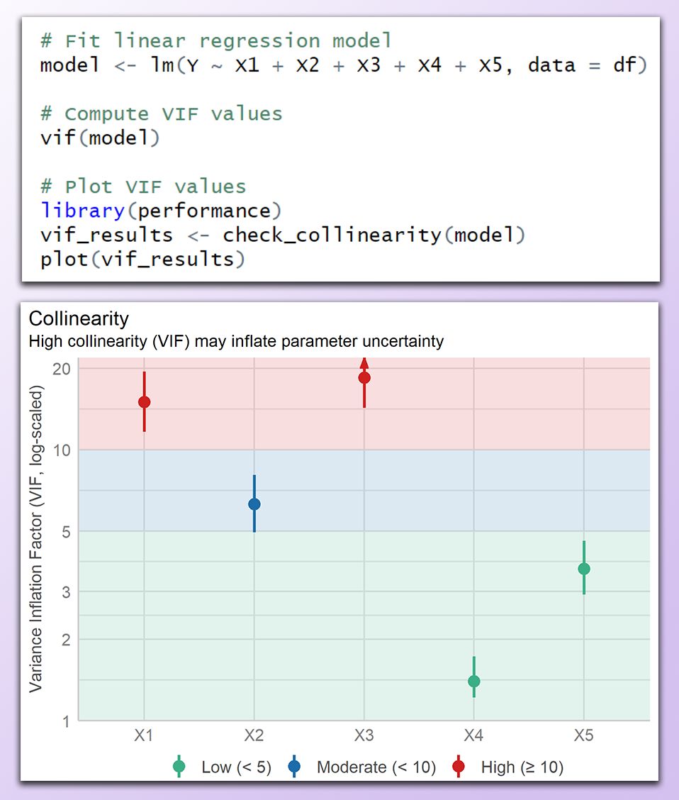
✔️ A VIF below 5 suggests low multicollinearity, while values between 5 and 10 indicate moderate correlation that may require attention. A VIF above 10 is considered problematic, as it can significantly distort regression estimates.
✔️ Addressing high VIF values improves model stability. Strategies include removing redundant variables, combining correlated predictors, using Principal Component Analysis (PCA), or applying regularization techniques like ridge regression.

❌ VIF only detects linear relationships, meaning nonlinear dependencies may go unnoticed. Alternative methods, such as Generalized Additive Models (GAMs) or mutual information, can capture nonlinear correlations.
❌ VIF does not indicate whether collinearity affects the target variable, so it should be used alongside domain knowledge and model evaluation techniques. Even if VIF is high, multicollinearity is only a concern if it negatively impacts model predictions or inference.

The image below was created in R and shows a VIF plot categorizing predictor variables into low (green), moderate (blue), and high (red) multicollinearity. Variables X1 and X3 have high VIF values, indicating strong collinearity that should be addressed before interpreting the model.

🔹 In R, vif() from the car package computes VIF, while check_collinearity() from performance provides visualization. Ridge regression with glmnet can mitigate multicollinearity by applying regularization.
🔹 In Python, variance_inflation_factor() from statsmodels.stats.outliers_influence quantifies multicollinearity, and ridge regression with sklearn.linear_model.Ridge() helps stabilize estimates by penalizing large coefficients.

Looking to improve your regression models? Check out my online course on Statistical Methods in R! Check out this link for more details: https://t.co/7YQCRDKSPO

#datasciencetraining #StatisticalAnalysis #Rpackage #RStats #DataVisualization #R4DS

[The Scientific Lens @LensScientific]

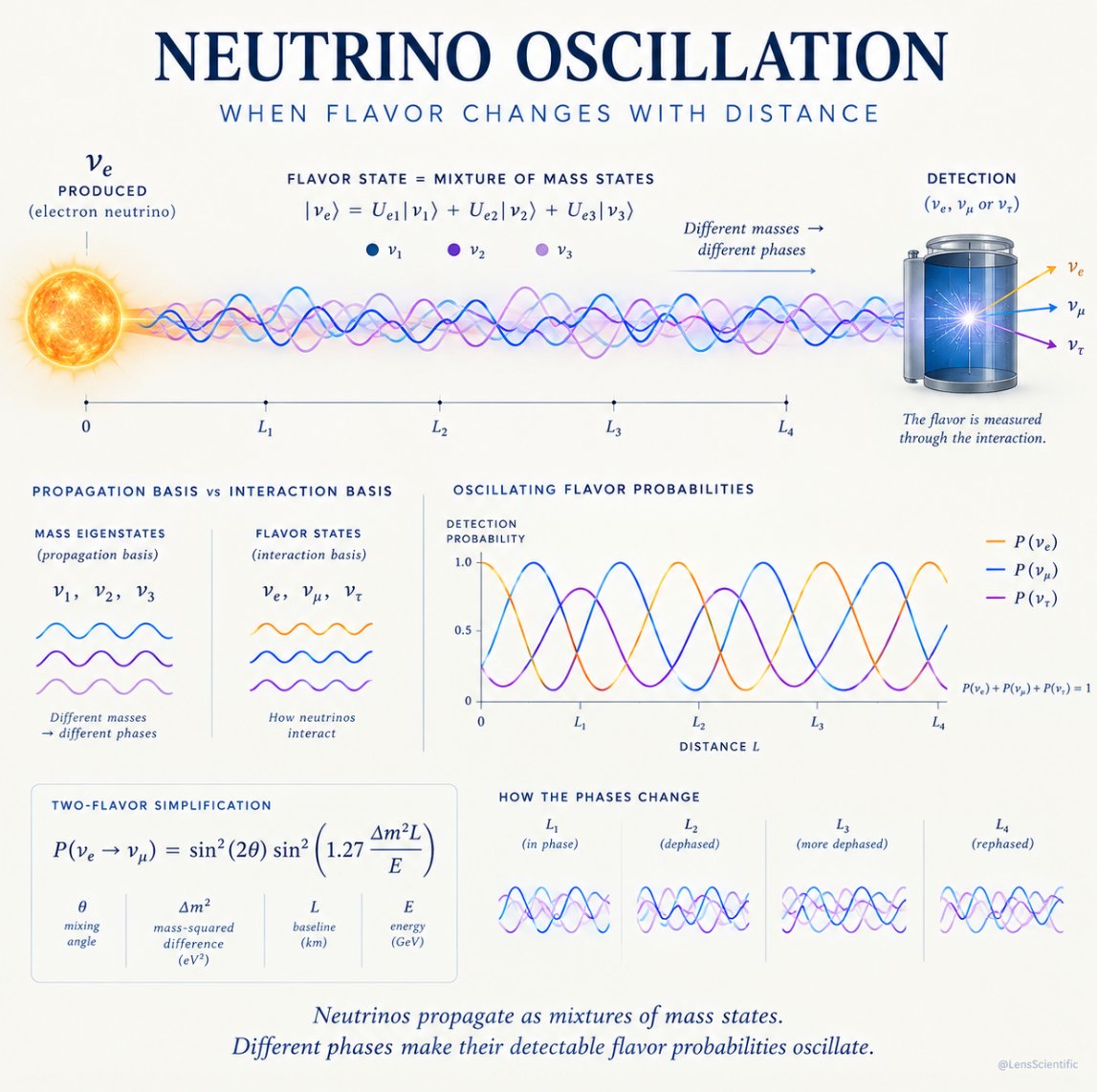
Neutrinos are born in one flavor, yet they can be detected as another.

As they travel, their mass states accumulate different quantum phases. These phases interfere, causing the probability of detecting an electron, muon, or tau neutrino to oscillate with distance.

[Architecture Presentation @arcpresentation]

Termites function as natural ventilation systems. Their galleries allow air to circulate continuously: hot air rises and exits, while cooler air enters to replace it. Some architects use this biomimetic principle to design buildings with internal ducts, air inlets in low areas, and upper exits. Continuous movement of air prevents heat from getting trapped and helps keep indoor spaces cooler. Combined with thermal mass, shade, and an appropriate opening design, this system can significantly reduce the need for mechanical cooling.

[The Scientific Lens @LensScientific]

A time crystal sounds like science fiction, but the idea is precise. In an ordinary crystal, atoms arrange themselves in a repeating pattern through space. A time crystal extends the idea to time: under a periodic drive with period T, a many-body quantum system can settle into a stable response with period 2T.

The drive repeats once. The system takes two cycles to return to its original state. This is called a subharmonic response, and it represents a breaking of discrete time-translation symmetry.

And no, it isn’t perpetual motion. The system is driven from the outside and does not create energy from nothing.

[The Scientific Lens @LensScientific]

The Navier–Stokes equations describe how fluids move under the influence of pressure, viscosity, inertia, and external forces.

They combine Newton’s second law with the physics of fluid deformation. The result is a set of nonlinear partial differential equations that can describe everything from air flowing around an aircraft to water moving through a pipe. At their core, they track how a fluid’s velocity and pressure change through space and time.

[Dreams N Science @dreamsNscience]

Nikola Tesla’s 1920 “valvular conduit” is a check valve with no moving parts.

Its asymmetric geometry simply makes flow far more resistant in one direction than the other.
A passive fluid diode that still fascinates physicists and engineers a century later.​​​​​​​​​​​​​​​​​​​​​​​​​​​​​​​​​​​​​​​​​​​​​​​​​​

🎥 physicsfun

[Mathematica @mathemetica]

How can a force weaker than a falling leaf still change a spacecraft’s orbit around the Sun?

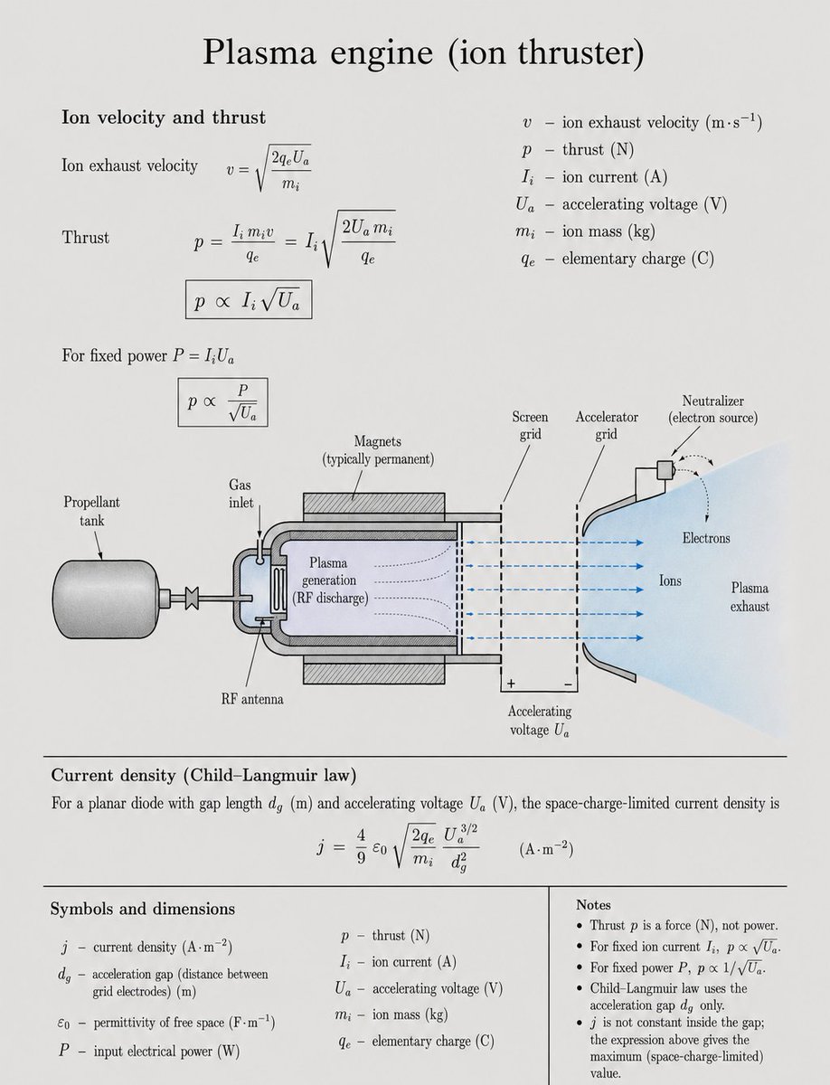
Ionize a trickle of xenon, apply voltage \(U_a\), and energy conservation fixes the exhaust speed:

v = √(2qₑUₐ / mᵢ)

because ½ mᵢv² = qₑUₐ.

Thrust is mass-flow times that speed. With ṁᵢ = Iᵢ mᵢ / qₑ you get

p = Iᵢ √(2Uₐ mᵢ / qₑ)  so  p ∝ Iᵢ √Uₐ.

Hold beam power fixed, P = IᵢUₐ, and the same relation flips:

p ∝ P / √Uₐ.

Higher voltage buys specific impulse I_sp = v / g₀ at the cost of raw force.

The current density you can actually pull is space-charge limited (Child–Langmuir):

j = (4/9) ε₀ √(2qₑ / mᵢ) · Uₐ³⁄² / d_g²

Those four relations flew Dawn to Vesta and Ceres, hold geostationary satellites on station, and will send probes farther on kilograms of xenon than chemical rockets can on tons.

A force too small to feel, integrated for years, rearranges the Solar System.

Which mission first made you trust specific impulse more than peak thrust?

[Physics Magazine @PhysicsMagazine]

Why does the superhydride LaSc₂H₂₄ outperform other high-pressure, high-remperature superconductors? It turns out that its scandium atoms modify the electronic structure, bridging a split in the superconducting gap that limits its rival LaH₁₀.

🔗 https://t.co/TVOBFTABcK

[Matheorems @matheorems]

A brain, a river, an ecosystem and your friend group are the same object in different colors.

They are networks G = (V, E): nodes for entities, links for relationships.
Degree kᵢ counts connections. Clustering Cᵢ measures triangles — how tightly neighbors link.
One language for proteins, neurons, drainage basins and society.

The map stays the same. Only the labels change.
Which system first made you see the graph underneath?

[The Scientific Lens @LensScientific]

Minkowski spacetime combines space and time into a single four-dimensional framework.

Every event is a point in this spacetime. The light cone then divides the universe around that event into three regions: the causal future, the causal past, and elsewhere, where no causal signal can reach. The cone is essentially a map of what can affect what, limited by the speed of light.

[Rosana Ferrero 📈📊🙌 @RosanaFerrero]

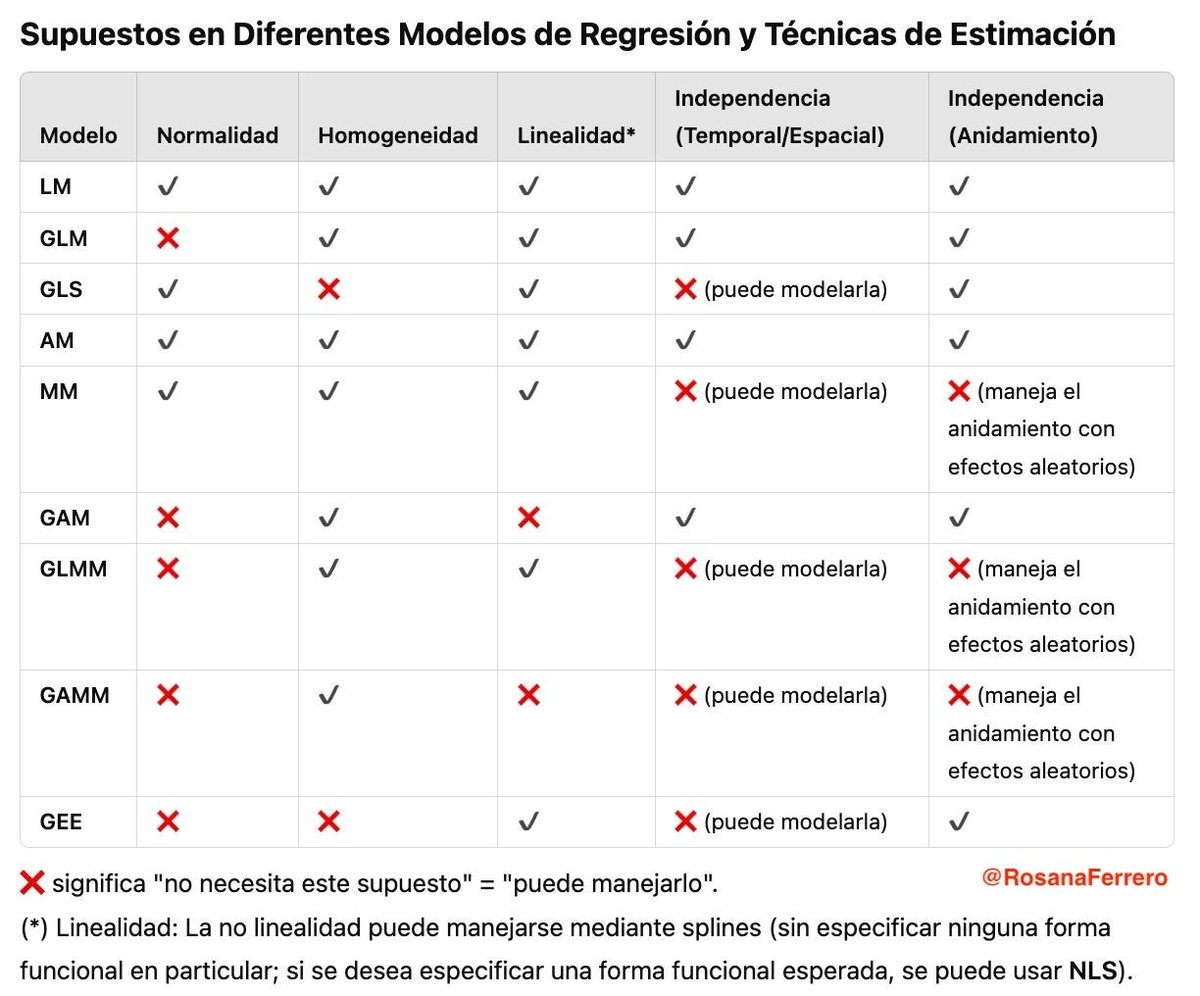
📊 ¿Qué modelo de regresión elegir? Este mapa se supuestos estadísticos resume de un vistazo qué supuestos exige (✓) y cuáles es capaz de perdonar o modelar (❌) cada gran familia de modelos de regresión.
Los modelos:👇🧵

#stats #datascience #cienciadedatos #estadistica #rstats

[The Scientific Lens @LensScientific]

Rusting is an electrochemical process. Iron loses electrons while oxygen is reduced, with moisture allowing ions to move. The familiar reddish-brown rust is a mixture of hydrated iron oxides and iron oxyhydroxides.

[Motorpasión @motorpasion]

La dinastía Maeda: cómo un padre y un hijo han dado forma a los legendarios diseños Kodo de Mazda https://t.co/QToAdC36Bo

[The Scientific Lens @LensScientific]

An electron orbital is not a path an electron follows around the nucleus. It is a quantum state described by a wavefunction, with |ψ|² giving the probability density of finding the electron.

The orbital type is set by the angular quantum number ℓ:
ℓ = 0 → s
ℓ = 1 → p
ℓ = 2 → d
ℓ = 3 → f

The principal quantum number n determines the shell. For a given n, ℓ can only range from 0 to n−1. That is why 3d exists, but 2d does not.

[Capo Estoico. @CapoEstoicoX]

8 Materias que estudian los hijos de los multimillonarios desde que aprenden a leer...

- Hilo -

[Computer Hoy @computerhoy]

Ubuntu en Android: así puedes llevar Linux en el móvil y olvidarte del PC https://t.co/NvqecCQ8sr

[Engineering Explained @Engineering67]

Why Pumps CANNOT Suck Water Deeper Than 10.3 Meters!

[Things Worth Knowing @Worth_Knowin]

Variable Frequency Drive (VFD) Working Explained .

[BBC News Mundo @bbcmundo]

"La generación sobria": por qué cada vez más jóvenes están reemplazando el alcohol por medicamentos para la ansiedad https://t.co/vaMznJk3gd

[ESA España @esa_es]

#LecturasDeVeranoESA 📖 - En enero descubrimos que la misión Sentinel-5P de @CopernicusEU
rastrea la contaminación atmosférica desde el espacio, lo que nos permite obtener una imagen más clara del aire que respiramos.
Pequeñas partículas de polvo y gotitas —«aerosoles»— flotan por todo el planeta. Pueden desencadenar asma, provocar lluvia ácida e incluso alterar el clima al absorber y dispersar la luz solar.