X

[Emrullah @emrullahai]

AKADEMİSYENLER VE DOKTORA ÖĞRENCİLERİNİN HEP KULLANDIĞI AMA HERKES BİLSİN İSTEMEDİĞİ SİTELER.

Bunu kaydedin mutlaka. Akademik anlamda sürekli ödeme yapmanıza gerek yok. Aşağıdaki siteler size fazlasıyla yetecek.

1. https://t.co/AiiUAUM75I
Dünyanın en büyük açık kütüphanesi. Profesörünüzün atadığı neredeyse her ders kitabı burada ücretsiz olarak mevcut.

2. https://t.co/lxrqkX8FtH
Akademik makaleler için arama motoru. En etkili araştırmaları bulmak için atıflara göre sıralayın.

3. https://t.co/rexxn41f8R
Akademik tez ve makale üretim motoru. Sıfır halüsinasyonla bölüm yazımı.

4. https://t.co/9AcMjHxGwm
Allen Enstitüsü tarafından geliştirilen yapay zeka destekli makale arama. Her atıfı bağlamında vurgular.

5. https://t.co/1pUSgSdS6D
Bir makaleyi girin, her ilgili çalışmayı bir grafik olarak haritalanmış görün. Uzmanların gerçekten birlikte okuduğu şeyleri ortaya çıkarır.

6. https://t.co/tHPqEh4Jfa
Bir yapay zeka araştırma asistanı. Herhangi bir soruyu sorun ve ana bulgularla birlikte yapılandırılmış makale tabloları alın.

7. https://t.co/iQBF4OKvAL
Binlerce makalenin sonuçlarını tek bir cevapta birleştirir. Kiraz seçmeyi önler.

8. https://t.co/FGPnpvrhZy
Makalelerin Spotify'si. Zaten okuduklarınıza dayanarak yeni araştırmalar önerir.

9. https://t.co/Hvs7besTv6
Atıf zincirlerini görselleştirir. Bir fikrin on yıllar süren araştırmalarda nasıl yayıldığını gösterir.

10. https://t.co/Pl3X0YIvIg
Hangi makalelerin herhangi bir iddiayı desteklediğini, çürüttüğünü veya bahsettiğini söyler. Saatlerce gerçeklik kontrolü yapmaktan tasarruf sağlar.

11. https://t.co/r7BhsKSHp7
200 milyon açık erişimli makale tek bir aranabilir indekste. Dünyanın en büyük ücretsiz akademik arşivi.

[Math is Sacred @mathissacred]

Stoke's Theorem - Visualization😍!

[Kafka @kfk_ai]

徐亦达教授（Prof Richard Xu），香港浸会大学数学系教授，“TadReamk Limited”创始人

他在 GitHub 上只有一个真正爆款项目：`machine-learning-notes`（9663 stars，1767 forks），一部 2000+ 页的机器学习、概率模型和深度学习的幻灯片合集，附带视频链接

除此之外的 13 个仓库，大多是无描述、无更新、无代码的“三无产品”。他拥有 5347 个 followers，但关注 0 人——绝对的知识输出者，社交黑洞

[灰狐 @huihoo]

自由图书《Calculus Early Transcendentals | 2021A》
626 pages, 彩色图文, CC 许可证，你可以下载 PDF 和 LaTex 文件
https://t.co/ivKxk60yvy

这是一本优秀的免费资源，能帮助你打下扎实的微积分基础
本书语言清晰易懂，同时又保持了适当的数学严谨性
书中包含丰富的例题和练习，既适合自学，也适合课堂教学

本书涵盖了广泛的主题，包括极限、导数、积分、数列、级数、微分方程和多元微积分等

这是一本开放教材，作者鼓励教师和学生通过注释、修订和重复使用来充分利用本书内容

[Antonio Lupetti @antoniolupetti]

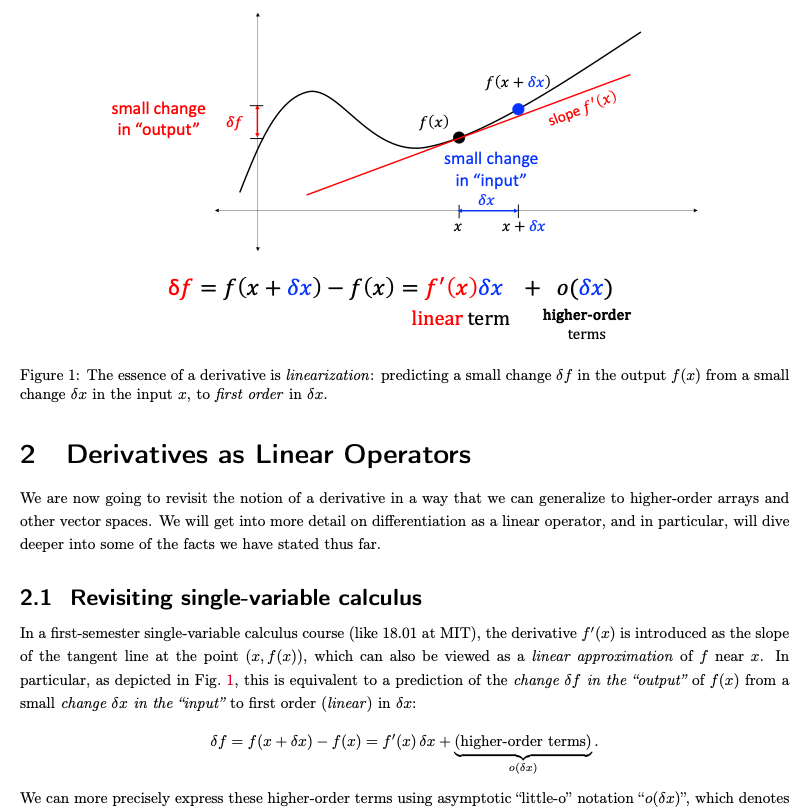
"Matrix Calculus for Machine Learning and Beyond" is an interesting set of free lecture notes for understanding the mathematics behind modern deep learning. It covers gradients, Jacobians, Hessians, matrix-valued functions, backpropagation, optimisation, and many of the mathematical structures used in machine learning and AI models.

One interesting aspect is that the material maintains a strong university-level rigour while remaining highly visual: the notes include numerous diagrams, graphs, geometric interpretations, and intuitive explanations of matrix calculus applied to neural networks.

It is a valuable resource not only for students studying machine learning, but also for anyone who wants to build a solid foundation in computational linear algebra and optimisation.

https://t.co/XsnReRHu35

[Joruno @wsl8297]

以前做数学、物理教学交互动画，Manim 这类专业工具几乎绕不开：LaTeX 公式渲染、镜头运动、动画编排，都得逐个搞定。

现在有了开源 AI 工具 Math-To-Manim：一句话描述，你就能直接生成完整的交互动画。

它会从概念拆解开始，循序搭建到目标主题，自动补齐 LaTeX 公式细节与镜头设计，把“写脚本、做动画”的流程一键自动化。

GitHub：https://t.co/cJfA0717l5

不止输出动画代码，还会生成完整的 LaTeX 学习笔记文档，并提供 55+ 个示例动画，覆盖物理、数学、计算机科学等方向。

使用也很直接：克隆仓库到本地，安装依赖，配置模型 API Key，在可视化界面输入描述，就能生成动画。

[一只小橘呀 @Ellieorange8]

数学系硕士强烈推荐的数学学习资源：awesome-math

其实真正高质量的数学教材、视频、题库，全被整理在一份 GitHub 清单里

Awesome Math，已获 14k+
它把代数、几何、分析、概率、数论等 30+ 领域
全部拆成体系化入口

📌 视频课 + 电子教材 + 练习工具
📌 甚至 MIT、哈佛学生的课程笔记
📌 持续更新，帮你省掉筛选时间

想用数学碾压所有人，直接收藏这份清单：
https://t.co/At3E4YFNbY

[Probability and Statistics @probnstat]

Teichmüller Space is a central object in geometry and complex analysis. It describes all possible geometric structures of a surface, up to smooth deformation. Originally developed in topology and Riemann surface theory, it studies how shapes can change while preserving intrinsic conformal properties.

In machine learning, Teichmüller geometry has become relevant in geometric learning and manifold-based representation. Many datasets lie on nonlinear manifolds rather than Euclidean space, and Teichmüller tools help understand shape-preserving embeddings, geometric feature extraction, and structured latent spaces.

In deep learning, it appears in geometric deep learning, graph embeddings, and shape analysis. Surface matching, medical imaging, 3D vision, and mesh learning often rely on conformal mappings closely related to Teichmüller theory.

In reinforcement learning, Teichmüller-inspired geometry can help in navigation on curved spaces, continuous control, and manifold optimization. The deeper idea is that learning often happens not in flat vector spaces, but on curved geometric structures, where understanding the geometry of deformation becomes crucial.

[Alec Helbling @alec_helbling]

In flow matching, a coupling determines how noise and data samples are paired during training.

The choice of coupling is important because it influences the geometry of trajectories at inference time.

The simplest choice is the independent coupling, where noise and data points are paired arbitrarily. This can lead to curved trajectories as the model averages over many conflicting pairings.

However, if we use optimal transport on batches of pairs, this leads to fewer ambiguous intersections that the model must resolve, leading to straighter trajectories at inference time.

[Alec Helbling @alec_helbling]

The Helmholtz decomposition is one of the fundamental results of vector calculus.

It says any well-behaved vector field can be split into two parts, one capturing sources and sinks through divergence, and one capturing rotation through curl.

[灰狐 @huihoo]

OpenRadioss
值得关注的开源工程软件生态，Fortran 核心驱动，AGPL-3.0 license
https://t.co/zQFjeXF0EN

Altair Radioss 是一款经业界验证的分析解决方案
可帮助用户评估和优化产品在动态载荷下的高度非线性问题的性能
解决复杂的非线性工程问题

30 多年来，众多机构一直使用 Altair Radioss 来简化和优化数字化设计流程，用快速高效的仿真取代成本高昂的物理测试，并加快设计优化迭代速度

2022年9月，Altair 推出 OpenRadioss 开源软件
旨在将全世界的专家和用户聚集在一起，使世界变得更安全、更环保

此项目可用于：
电池开发、轻质材料和复合材料、人体模型和生物材料、自动驾驶和飞行
以及通过虚拟测试完成汽车乘员安全性分析等技术

1991 年，全球首次汽车碰撞模拟实验就是使用 Radioss 软件完成的
用计算机模拟取代物理测试将带来巨大优势

数学、物理学、工程软件、高性能计算，对 Fortran 是依赖的

LLVM 项目也优先支持 Fortran，提供 Flang 编译器
Flang 是一款现代的 Fortran 编译器及其运行时环境
旨在生成高性能代码，并支持 Fortran 2023 以及所有官方 Fortran 标准
（甚至可追溯至 Fortran 77），包括许多广泛使用的扩展
Flang 支持 CPU 和 GPU 的 OpenMP 协议

学习使用开发 Fortran 软件，形成差异化优势，也是一种选择

[Mathelirium @mathelirium]

Final Lecture of our Statistical Mechanics Series.

Lecture 2 showed how we move from the Full Phase-Space Density

ρ(q₁, …, qₙ, p₁, …, pₙ, t)

to smaller statistical objects by integrating out variables we do not want to keep. That gives reduced descriptions like the One-Particle Density

f₁(q₁,p₁,t)

and the Two-Particle Density

f₂(q₁,p₁,q₂,p₂,t)

This was the simplification.

Now comes the catch.

If the Full Density obeys Liouville’s Equation, the reduced densities do not evolve independently. The equation for one level depends on the next one and this is referred to as the BBGKY hierarchy.

The One-Particle Density depends on the Two-Particle Density.
The Two-Particle Density depends on the Three-Particle Density.
And the chain keeps going.

That happens because particles interact. Once one particle feels the rest, one-particle information is no longer enough. Correlations enter, and the lower level is fed from above.

If the full Hamiltonian is

H = Σᵢ pᵢ²/(2m) + Σᵢ U(qᵢ) + (1/2) Σᵢ Σⱼ≠ᵢ Φ(qᵢ − qⱼ)

then reducing the full density does not make the interaction terms disappear. It leaves behind coupling to higher-order reduced densities. So, schematically,

∂f₁/∂t + transport of one particle = interaction term involving f₂

and more generally the heirarchy is such that

∂fₛ/∂t + s-particle transport = interaction term involving fₛ₊₁

Therefore, Lecture 3 is really about the price of reduction. We simplify the description, but the information we remove comes back as coupling to higher-order correlations.

So, how do you actually compute anything if every level depends on the next one?

This is the so-called Closure Problem.

To make the hierarchy usable, you need an extra assumption that cuts the chain. You replace the exact higher-order object by an approximation in terms of lower-order ones. The most basic example is a factorized closure at the pair level, where the exact correlated Two-Particle Density is replaced schematically by a product of One-Particle Densities:

f₂(q₁,p₁,q₂,p₂,t) ≈ f₁(q₁,p₁,t) f₁(q₂,p₂,t)

That approximation is not exact. It throws away part of the correlation structure. But it gives you something the raw hierarchy does not... a closed equation for the lower-level description.

That is why closure matters so much. Without it, the hierarchy is exact but open. With it, the theory becomes approximate but usable.

Thus, the combined point of this final Statistical Mechanics post is simple.

First, reduced descriptions are not closed because interactions generate correlations across levels.
Second, if you want a workable Kinetic Theory, you must close the hierarchy by approximating those higher-order correlations.

It is the bridge from formal many-body mechanics to equations people can actually solve.

In the render, that is exactly the story you are seeing. The first part shows the hierarchy itself: one reduced level feeding the next, with lower descriptions inheriting structure from higher ones. The second part shows the closure step where the exact correlated pair level is replaced by a factorized ansatz, and that approximation gives back a closed one-particle description. That is, the animation moves from dependence to approximation, and from approximation to solvability.

#StatisticalMechanics #BBGKY #ClosureProblem #KineticTheory #PhaseSpace #ReducedDistribution #HamiltonianMechanics #MathematicalPhysics #Mathematics #Physics

[Philosophy Of Physics @PhilosophyOfPhy]

In physics tesseract is used to model higher dimensional spaces, such as in theoretical physics, cosmology (e.g., studying dark energy), and general relativity.

[JJ @JosephJacks_]

One equation generates all of reality. The Lagrangian ℒ = T − V — kinetic minus potential energy — is the seed. Feed it a symmetry group and it tells you which universe you get. U(1) gives you light. SU(3) gives you confinement. SU(2)×U(1) gives you mass via the Higgs. The entire Standard Model — every force, every particle, every interaction — is just one Lagrangian density with the gauge group SU(3) × SU(2) × U(1). I made this infographic to show what most physics education never makes visual: the deep structure is a single equation that branches into all of physical reality based on which symmetry you choose. Nature doesn’t pick forces. It picks symmetries. The forces are consequences.

[Philosophy Of Physics @PhilosophyOfPhy]

This is one of the best Visual Explanation of how LLMs actually work.

[Alec Helbling @alec_helbling]

Divergence and curl are complementary concepts from vector calculus.

Divergence quantifies the rate at which a field flows outward from a point and curl represents rotation.

A single vector field can have both divergence and curl, leading to an outward spiral pattern.

[KK.aWSB @KKaWSB]

拉里·埃里森：“世界上每一个大型语言模型——ChatGPT、Gemini、Grok、Claude、Llama——每一个都使用完全相同的数据进行训练：互联网上的公共数据。所以它们都会趋于一致。它们都会变得一样。唯一能让它们大幅提升的方法，就是用私有数据来训练它们——你们的私有数据。这就是真正价值所在的地方。”

[Zara Zhang @zarazhangrui]

https://t.co/QfJPQXi1cO