Yanyan Xu

Working on Urban Science and AI for Science.
Associate Professor@AI Institute, SJTU

[Nature Computational Science @NatComputSci]

📢Out now! @yxu_mit, @martikagv, and colleagues introduce neuroGravity, a model to reconstruct mobility networks in data-scarce regions. https://t.co/OY9G0bwQRe

🔓https://t.co/NY7TUSwGB7

[Jorge Bravo Abad @bravo_abad]

Physics-informed GNNs for mobility in data-poor cities

Human mobility shapes traffic, access to services, epidemics, pollution exposure and socioeconomic opportunity. But mobility data are uneven, where surveys or mobile-phone records are scarce.

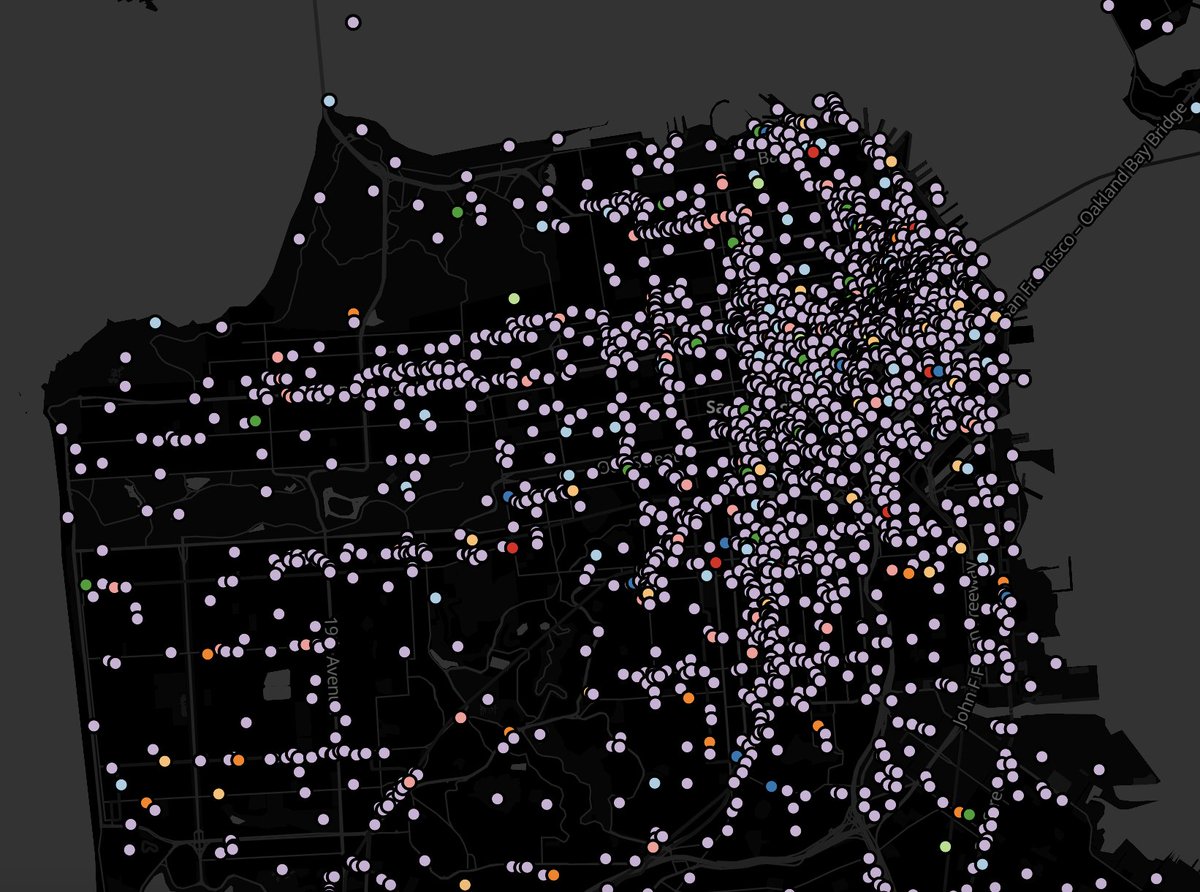
Jinming Yang and coauthors address this gap with neuroGravity, a physics-informed model that reconstructs mobility networks from sparse observations and public data. It keeps the classical gravity model, where flows depend on population and distance, but places it inside a GNN that learns from population, OpenStreetMap features, land use, roads and points of interest.

This is not just another black-box model. A learned “meta-Gravity” component first produces a physically grounded estimate of flows, then an edge-enhanced graph transformer refines it. The model does not need to rediscover that larger places attract people and that distance matters. It can focus on deviations from that simple law.

In Boston, neuroGravity reconstructs 51,000 OD flows with R² = 0.77 when only about 1% of internal links are observed. Across cities, it outperforms gravity models and standard GNN baselines, especially where data-driven models are most vulnerable.

The learned embeddings also capture socioeconomic structure without being trained on income. Combined with OpenStreetMap features, they help predict carbon footprint, nitrogen dioxide and radius of gyration. A model trained to reconstruct movement also learns how the city is socially and functionally organized.

A model trained on Boston can generate zero-shot mobility networks for Los Angeles, San Francisco Bay Area, Bogotá and Rio de Janeiro. Transferability is linked to spatial income segregation: similar segregation patterns make cities easier to transfer between. The authors use this insight to estimate mobility proxies for over 1,200 cities worldwide.

This shows what physics-informed ML can do when measurements are scarce. The same logic is relevant to R&D pipelines in drug discovery, materials development, energy and biotechnology: encode what is known, learn missing corrections, and use transferability diagnostics to decide where a model can be trusted.

Paper: Yang et al., Nature Computational Science (2026) | https://t.co/nUX4nCnQfo

[Jorge Bravo Abad @bravo_abad]

Chemma: Accelerating organic chemistry synthesis with Large Language Models (LLMs)

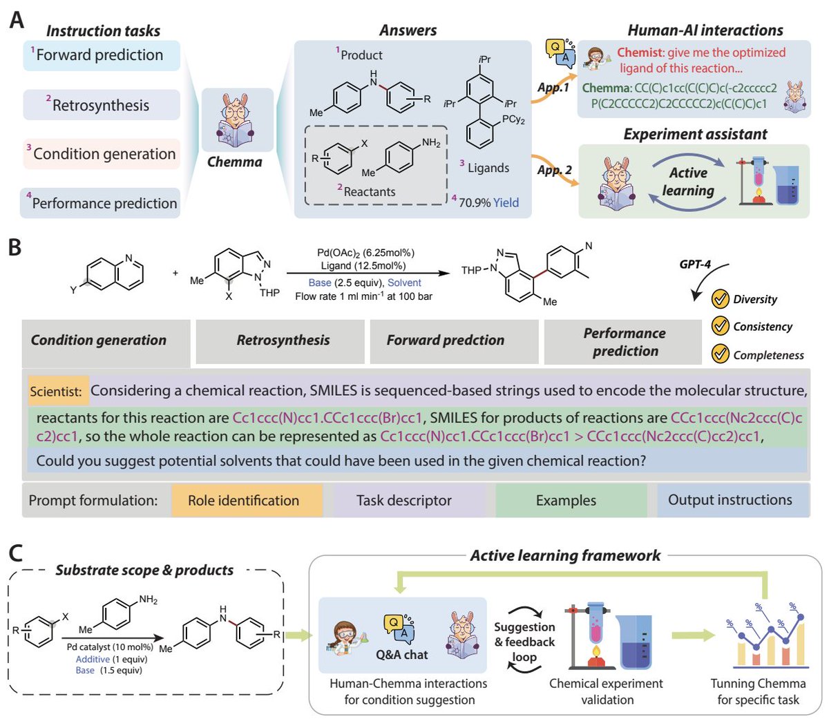
In a recent study published in Nature Machine Intelligence, Yu Zhang and coauthors introduce Chemma, an advanced Large Language Model fine-tuned from LLaMA-2-7B using an extensive dataset of 1.28 million chemical Q&A pairs.

Chemma significantly surpasses existing approaches in tasks such as single-step retrosynthesis, yield prediction, and reaction-space exploration. Remarkably, it accelerated the optimization of a previously unreported Suzuki–Miyaura reaction, achieving high yields within just 15 experimental runs via an innovative human–AI collaboration.

This pioneering research underscores the transformative impact AI can have on chemistry, driving more efficient, intelligent, and autonomous chemical synthesis.

Paper: https://t.co/RdDRGeBH7l

[NetScience @net_science]

Human mobility prediction with causal and spatial-constrained multi-task network https://t.co/cGn7ZrkTzI

[Selçuk Korkmaz @selcukorkmaz]

A Simple Guide on Quantile Regression

🧵1/ Introduction to Quantile Regression 📈
Ever noticed how average predictions (like mean) might not capture the entire story of your data? Enter Quantile Regression (QR)! Instead of focusing just on the mean, QR looks at various quantiles (percentiles) of the response variable.

2/ Traditional vs. Quantile Regression 📊
Traditional linear regression predicts the mean of the dependent variable. But what if we're interested in, say, the median? Or the 90th percentile? QR allows us to model these specific quantiles, providing a fuller picture of the data's distribution.

3/ Why use Quantile Regression? 🤔
• To understand the relationship at various points (quantiles) of your dependent variable.
• Highly robust to outliers.
• Helpful when the residuals of a linear model aren’t homoscedastic (i.e., they have non-constant variance).

4/ How does it work? 🛠️
QR minimizes the sum of weighted absolute residuals, unlike least squares regression which minimizes squared residuals. By changing the weights, we target different quantiles.

5/ When to use Quantile Regression? 📅
• When you suspect heteroscedasticity.
• To analyze the impact of variables at different parts of the distribution.
• When interested in high or low extremes (e.g., what factors influence the top 10% of incomes).

6/ Visualization Power 🌈
Plotting several quantile regressions together can give a more holistic view of the data relationship. For instance, seeing how the effect of education on income changes across the income distribution.

7/ Limitations 🚫
• Can be computationally intensive for large datasets.
• Interpretation might be less intuitive than mean-focused methods.

8/ In Conclusion 🎓
Quantile Regression offers a versatile tool to understand relationships in your data that go beyond the average. It shines a light on the entire distribution, allowing for richer insights.

9/ Further Reading 📚
For those keen on diving deeper, many statistical packages, like R's quantreg, offer tools to implement and visualize QR. #Rstats

10/ Liked this thread? 🌟
Feel free to like, retweet, and share your experiences with Quantile Regression below! #Statistics #DataAnalysis #DataScience #QuantileRegression

[Brandon liu bsky.app/profile/bdon.org @bdon]

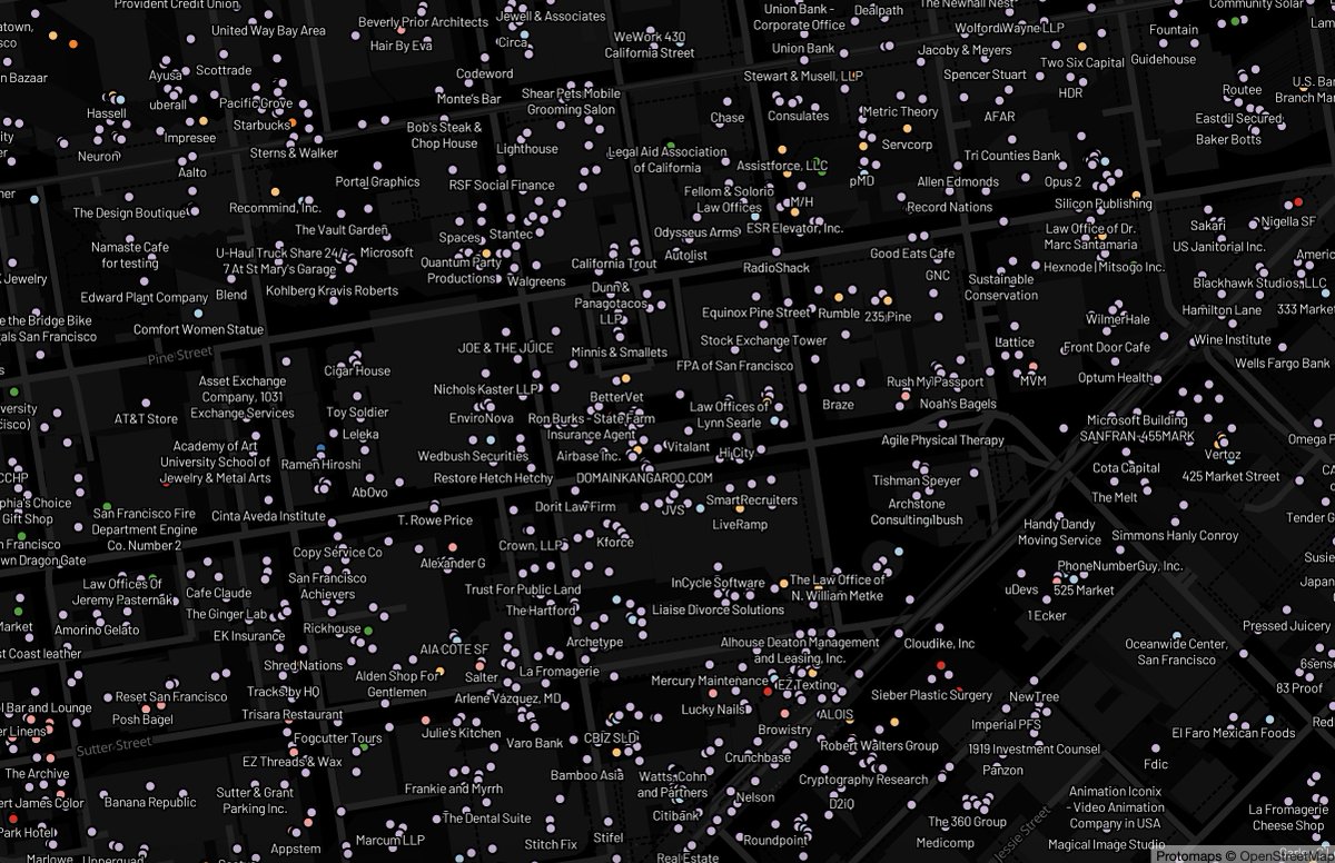
All @OvertureMaps places - 60 million of them - displayed in @maplibre with a 3.7GB tile archive:

https://t.co/qqo0003kgn

instructions https://t.co/0ZC0wg4DqC

2 steps
@duckdb parquet -> CSV
@felt tippecanoe CSV -> pmtiles

Thanks @Maxxen_ @opencholmes for the tips!

[Nature Computational Science @NatComputSci]

Our July issue is now live! Our cover highlights the exciting field of human mobility and how computational science can help advance this area.

👉https://t.co/53QQLREPLs

[Centre for Cities @CentreforCities]

Spanish cities, unlike Britain’s, are typically dominated by a mid-rise urban form, bringing economic benefits 🌆

#Barcelona, for example, is denser and has far greater transport accessibility than large UK cities 🇬🇧🇪🇸

Read the blog for more 📝🔽
🔗https://t.co/EdzODuSj4Q

[Gabriel Peyré @gabrielpeyre]

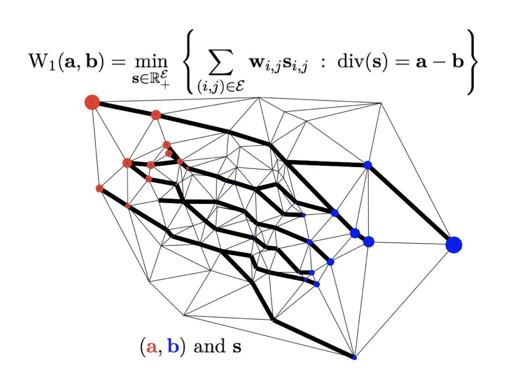
The Wasserstein-1 distance (which is a norm!) between histograms on graphs is equivalent to a min-cost flow. Bold black indicates edges where mass is flowing. https://t.co/tt2QjfnmRd

[Bloomberg CityLab @CityLab]

How much space do major US cities dedicate to car parking? Explore these 50 maps https://t.co/kSr4cI8oFC

[Gabriel Peyré @gabrielpeyre]

Comparing probability distributions: Csiszár f-divergences measure « vertical » displacement of mass, whereas dual norm of smooth functions rather measure « horizontal » displacements. https://t.co/XI2u19GlTj

[Tatsunori Hashimoto @tatsu_hashimoto]

We know that language models (LMs) reflect opinions - from internet pre-training, to developers and crowdworkers, and even user feedback. But whose opinions actually appear in the outputs? We make LMs answer public opinion polls to find out: https://t.co/wv3F6TOnwe

[Nature Human Behaviour @NatureHumBehav]

Early morning classes are associated with lower attendance, shorter sleep, and poorer academic achievement: https://t.co/8XCRTJNF5C

[Gabriel Peyré @gabrielpeyre]

Adding an independent Gaussian variable is the same as doing a heat diffusion on the density. https://t.co/CK4cUaON77

[Gabriel Peyré @gabrielpeyre]

Schrodinger’s problem is an approximation (regularization using diffusion) of the Optimal Transport problem. https://t.co/3nwtDvFOgJ

[Marta C. Gonzalez @martikagv]

Our new paper is out. It combines percolation theory with the macroscopic fundamental diagram https://t.co/h7jLhjBC2s

[Jean de Nyandwi @Jeande_d]

AI Research Experience - Harvard CS197

AI Research course and book that teaches how to do cutting-edge research, research workflows, and using tools commonly used in AI research(like PyTorch, Lightning, Hugging Face, and more).

Course book: https://t.co/0gMfZLaAnV

[Zhu Liu @LiuzhuLiu]

Carbon Monitor global CO₂ emissions updates for full year 2022:
Global CO2 increased by +1.6% in 2022 (+8.0% than 2020, and +2.1% than 2019)
China -1.3%
US +3.5%
EU+UK +2.4%
India +7.1%
Japan:+2%
Data download https://t.co/o66syeqt8o

[Gabriel Peyré @gabrielpeyre]

Various discrepancies between 1D probability distributions are derived from the cumulative function. They all share the good taste to control the convergence in law (thanks to the integration). https://t.co/p1fRlpQsvN https://t.co/YQAjvmShmv

[Rafael H. M. Pereira 🚡 Urban Demographics @UrbanDemog]

Great paper by @npalomin & @citygeographics looking at network-based metrics to examine the allocation of streetspace between pedestrians and vehicles https://t.co/i1Xcr2csjO Very glad to see it published in our SI Advances in Spatial and Transport Network Analysis on @envplanb