Pakay

[Pakay @Pakay20]

A Whole New World - Peabo Bryson and Regina Belle https://t.co/jViYqVEf3l ผ่าน @YouTube

[Fermat's Library @fermatslibrary]

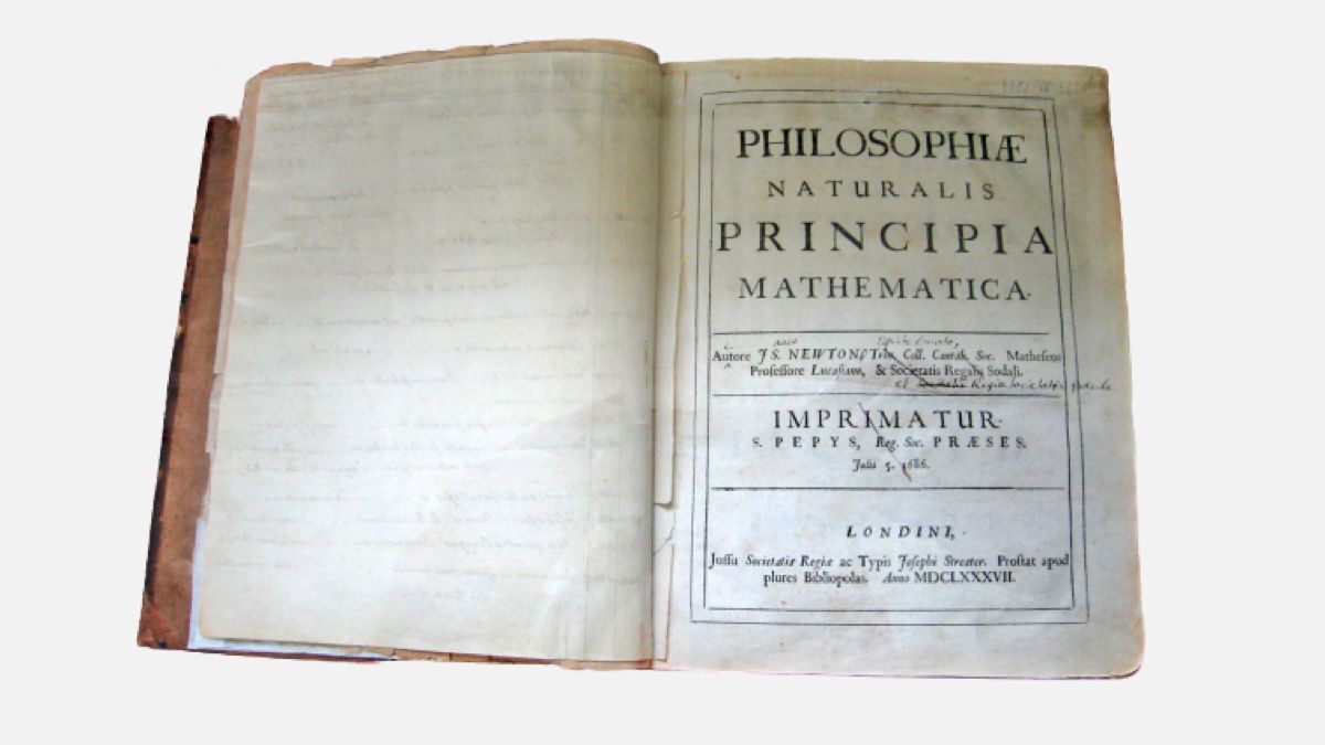
On this day in 1687, Newton’s Principia was published, arguably the most important science book ever printed.

The Royal Society couldn’t fund the printing since they’d spent their entire budget on a book about fish. Edmond Halley paid for the Principia out of his own pocket.

[Philosophy Of Physics @PhilosophyOfPhy]

Quantum mechanics did not merely add new equations to physics. It changed what physicists believed reality could be.

Energy became quantized. Light and matter refused to remain only particles or only waves. Superposition replaced a single definite state with several possible outcomes. Heisenberg showed that uncertainty is not simply poor measurement, but part of the structure of nature itself.

Probability entered the foundations of physics. Entanglement revealed correlations with no classical equivalent. Quantum statistics explained why atoms have structure, why chemistry works, and why ordinary matter does not collapse.

These ideas are strange, but they are not philosophical decoration. Together, they form one of the most precisely tested frameworks in science.

Quantum mechanics taught us something deeply unsettling and beautiful.

"Nature is not required to behave according to the categories human intuition finds comfortable."

[Cliff Pickover @pickover]

“Reality in Layers.” The Stratified Cosmos.

I created this diagram, stimulated by https://t.co/tN8v8WAmSV

[Fermat's Library @fermatslibrary]

"If I were to awaken after having slept for a thousand years, my first question would be: Has the Riemann hypothesis been proven?" - David Hilbert

[Massimo @Rainmaker1973]

Scientists have created one of the most detailed 3D reconstructions of a human cell (eukaryotic cell) ever produced.

This groundbreaking model, often termed a "Cellular Landscape Cross-Section Through a Eukaryotic Cell," combines data from X-ray tomography, nuclear magnetic resonance (NMR), and cryo-electron microscopy to map molecular structures in extreme detail.

[Mathematica @mathemetica]

Greek letters pack precise meanings into single characters that scientists and engineers use to keep equations clear and concise.

They represent concepts like angular acceleration with alpha, beta radiation with beta, photons and the Lorentz factor with gamma, changes with delta, damping with zeta, efficiency with eta, angles with theta, conductivity with kappa, wavelength with lambda, friction with mu, random variables with xi, the circle ratio with pi, density with rho and stress with sigma.

These symbols come into play when teams calculate friction coefficients with mu during tire testing or assess material stress with sigma in aerospace component design.

[Massimo @Rainmaker1973]

A step-by-step look at how photosynthesis works

[ScieVision @scievision369]

The Quantum State of a Qubit ✍️

A classical computer bit is like a coin lying flat on a table, either heads or tails, zero or one, with no uncertainty. A qubit is more like a coin spinning in the air; it truly embodies both possibilities at once. This isn’t because we are unsure of which side it will land on, but because while it's spinning, it is neither one thing nor the other. When you measure it, it settles into a definite outcome like a spinning coin that eventually lands. Until that moment, it exists in a superposition of both zero and one, with specific proportions of each part of its physical state.

The most fascinating idea in this diagram is the Bloch sphere, a simple-looking ball that maps every possible state a single qubit can have. The north pole of the sphere represents the state of definitely zero, the south pole represents definitely one, and every other point on the surface represents a different quantum superposition, a different mix of the two. The red arrow pointing from the center to the surface shows the qubit's state, and everything about the qubit's physics is encoded in the direction that arrow points. How much the arrow tilts tells you the measurement probabilities: an arrow pointing straight up means you will definitely measure zero, straight down means definitely one, and pointing sideways along the equator means a perfect fifty-fifty chance. Importantly, the arrow always reaches the surface, never sitting inside the sphere. A qubit in a perfectly controlled quantum state always lives on the surface. If it drifts into the interior, it means the quantum information has been damaged by unwanted interactions with the environment, which is why building real quantum computers is so challenging.

The second piece of information in the qubit's state is the phase, which is the horizontal rotation angle of the arrow around the vertical axis of the sphere. This is where things get truly strange. Two qubits can sit at the same height on the sphere, giving them the same measurement probabilities, but they can face different directions horizontally. While this difference is completely invisible if you measure either qubit directly, it becomes crucial when quantum states combine and interfere. Just like waves on water, where crests meeting crests create bigger waves and crests meeting troughs cancel out, quantum states with different phases interfere when combined through quantum operations. A quantum algorithm is essentially a carefully arranged sequence of these interferences, designed so incorrect answers cancel out while correct answers reinforce certainty. Every quantum gate, every operation in a quantum computer, corresponds to a physical rotation of the Bloch sphere, spinning the arrow from one direction to another. Designing a quantum algorithm is like choreographing a precise sequence of rotations. The entire power of quantum computing comes down to manipulating these two angles: one controlling what you see when you measure and the other controlling how states interfere, for a single arrow pointing at the surface of an ordinary sphere.

[Math is Sacred @mathissacred]

Understand😊! Euler's Formula.

[Infinite Logiz @Infinite_Logiz]

Taylor Series

[Cliff Pickover @pickover]

Mathematics.

The formula for the volume of a pyramidal square frustum appeared in ancient Egyptian mathematics in what is called the Moscow Mathematical Papyrus, written in 13th dynasty (1850 BC).

a and b are the base and top side-lengths; h is height. https://t.co/nAGkJ2ojUk

[Mathematica @mathemetica]

The golden ratio φ ≈ 1.618 defines the side proportions in the golden triangle.

Defined as φ = (1 + √5)/2, it satisfies the equation φ² = 1 + φ and equals the limit of ratios of successive Fibonacci numbers F_n.
Binet's formula expresses these numbers exactly using φ and its conjugate. The ratio also appears as the infinite continued fraction 1 + 1/(1 + 1/(1 + ⋯)) and produces a self-similar spiral by repeated subdivision of the triangle.

It is used to describe the efficient arrangement of seeds in sunflower heads.

[Mathematica @mathemetica]

Taylor series expand any smooth function around a point a using its derivatives at that point.

The formula is f(x) = Σ_{n=0}^∞ f^{(n)}(a)/n! (x-a)^n.

The graphic defines the components on the left and shows on the right how the linear (blue, n=1), quadratic (green, n=2), cubic (purple, n=3) and higher (orange) approximations approach the red curve y=f(x) near a. Color-coded terms below match the orders from constant to higher.

In real life, it is used to approximate functions in physics, engineering calculations, and computer algorithms for efficient evaluations.

[Mathematica @mathemetica]

Biological neuron compared to the artificial neuron used in neural networks.

- The top shows a biologic neuron: dendrites receive signals, the cell body processes them, the axon transmits the signal, and terminals pass it onward.
- The bottom shows an artificial neuron: inputs x₁ to xₙ are weighted by w₁ to wₙ, summed with bias B, then passed through activation function f to produce output. This model is the basis for artificial neural networks.

It drives applications such as image classification in social media and voice recognition in virtual assistants.

[Cosmos Archive @cosmosarcive]

This wheel is a clean, complete reference that connects every core formula for Ohm’s Law and electrical power in one visual.

P = power (watts)
V = voltage (volts)
I = current (amps)
R = resistance (ohms)

The relationships shown:

V = I × R
P = V × I
R = V / I
P = I² × R
P = V² / R
I = √(P / R)
V = √(P × R)

It lays out the full set of calculations clearly so you can move between voltage, current, resistance, and power.

[Math Files @Math_files]

Proof that πᵉ < eᵖⁱ

[Physics In History @PhysInHistory]

The Fourier series is a way to represent any periodic function as a sum of simple sine and cosine waves.

In essence, it breaks down complex signals into a combination of basic trigonometric functions, making it a powerful tool in mathematics, physics, and engineering for analyzing waveforms, heat transfer, vibrations, and more.

📹 Credit : mathswithmuza

[Mathsrick @mathsrick_]

A few matrices, a strange-looking equation, and a prediction that rewrote physics.

The Dirac equation remains one of the most beautiful examples of mathematics uncovering reality.

[Cosmos Archive @cosmosarcive]

Johannes Kepler discovered that planets move around the Sun in elliptical orbits, not perfect circles.

r = ℓ² / [m²μ(1 + e cos θ)]

This relation gives the distance of a planet from the Sun at any point in its orbit and became one of the foundations of celestial mechanics.