Totozy Kely

Just sharing some useful stuff.

[Concretum Research @ConcretumR]

Two weeks ago, our paper "The Volatility Edge: A Dual Approach for VIX ETNs Trading" was awarded 5th place at the @quantpedia Awards 2026.

We've now published a companion article covering the core concepts behind the strategy, including:

1️⃣ The volatility risk premium
2️⃣ From Options to VIX ETNs
3️⃣ Signal construction and regime detection
4️⃣ Dynamic position sizing
5️⃣ Strategy automation with Python in @IBKR

The article also includes a public Google Colab notebook that demonstrates the full workflow from signal generation to execution.

Links to the article, research paper, and notebook in first comment 👇.

[Concretum Research @ConcretumR]

Can you replicate the returns of one of the legends of the trend-following industry?

Just published.

We use 25 years of futures data and 4,320 synthetic CTAs to reverse-engineer the trading rules behind Paul Mulvaney.

The rules look simple.

The outcome is not.

Link in the comments 👇

[Concretum Research @ConcretumR]

How to build a complete futures price database across 100+ markets

Following strong demand from our readers and followers, we’ve decided to share a Python procedure to construct a comprehensive futures dataset using Norgate Data.

It’s a robust and reliable source, with coverage for some markets going all the way back to the 1980s, making it particularly valuable for long-horizon research and systematic strategy development.

Full details in the first comment 👇🏻

[A @BenP_np]

¿Cómo calculamos la volatilidad implícita de las opciones? La respuesta a eso cambió.

Cualquiera que haya armado un Excel o programa para valuar por Black-Scholes, o se haya puesto a revisar las fórmulas detrás de la planilla, se habrá dado cuenta de que mientras existe una fórmula cerrada para el precio de las opciones y para las griegas, a la hora de calcular la volatilidad implícita hay que optimizar: usar solver, un script en VBA o una función que encuentre numéricamente la volatilidad implícita que resuelva la fórmula con el resto de inputs conocidos.

Esto pasa porque Black-Scholes va para un solo lado. Le metés VI, strike, spot, tasa y tiempo, y te devuelve el precio. Pero en la práctica vos tenés el precio que ves en pantalla y querés saber a qué VI opera. Y para eso, durante 50 años, no quedó otra que iterar: tirar un valor, ver qué precio da, ajustar, volver a probar. Newton-Raphson, bisección, el Solver de Excel, etc.

Hace unas semanas salió un paper que parece resolver esto con una fórmula cerrada. Sale hilo 👇

(1/5)

[Quant Beckman @quantbeckman]

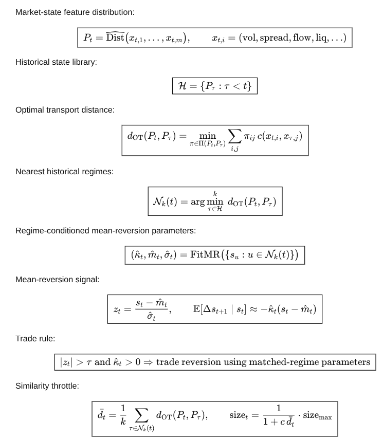
Use optimal transport distance to match today against historical days with similar volatility, liquidity, spread, flow, and cross-asset structure. The closest historical states define the regime library for calibration.

[Quant Beckman @quantbeckman]

This keeps the full curve shape instead of reducing the day to scalar features like close-to-close return or total volume. Learn the typical peer-group curve shape and measure today’s functional deviation from it. Trade when one asset’s curve becomes abnormally different from its peer-group shape.

[Quant Beckman @quantbeckman]

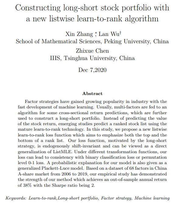
In alpha mining, thousands of features can look predictive by chance. Knockoff filters create synthetic copies of features that preserve dependence structure but carry no true signal. A real feature must beat its knockoff to be selected, which controls the false discovery rate. This keeps rare-edge hunting from becoming uncontrolled multiple testing.

[Matias Scalbi @MatiasScalbi]

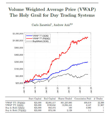
🔥 VWAP "The Holy Grail for Day Trading Systems"

Buscando papers para estrategias encontré este, el cual creo que a muchos de ustedes les puede interesar (en especial al amigo @OleosCapital)

Describe la estrategia a detalle para aplicarla en el Nasdaq

Si quieren que se los comparta completo, mandenme MD y les paso el archivo

[Łukasz Olejnik @prywatnik]

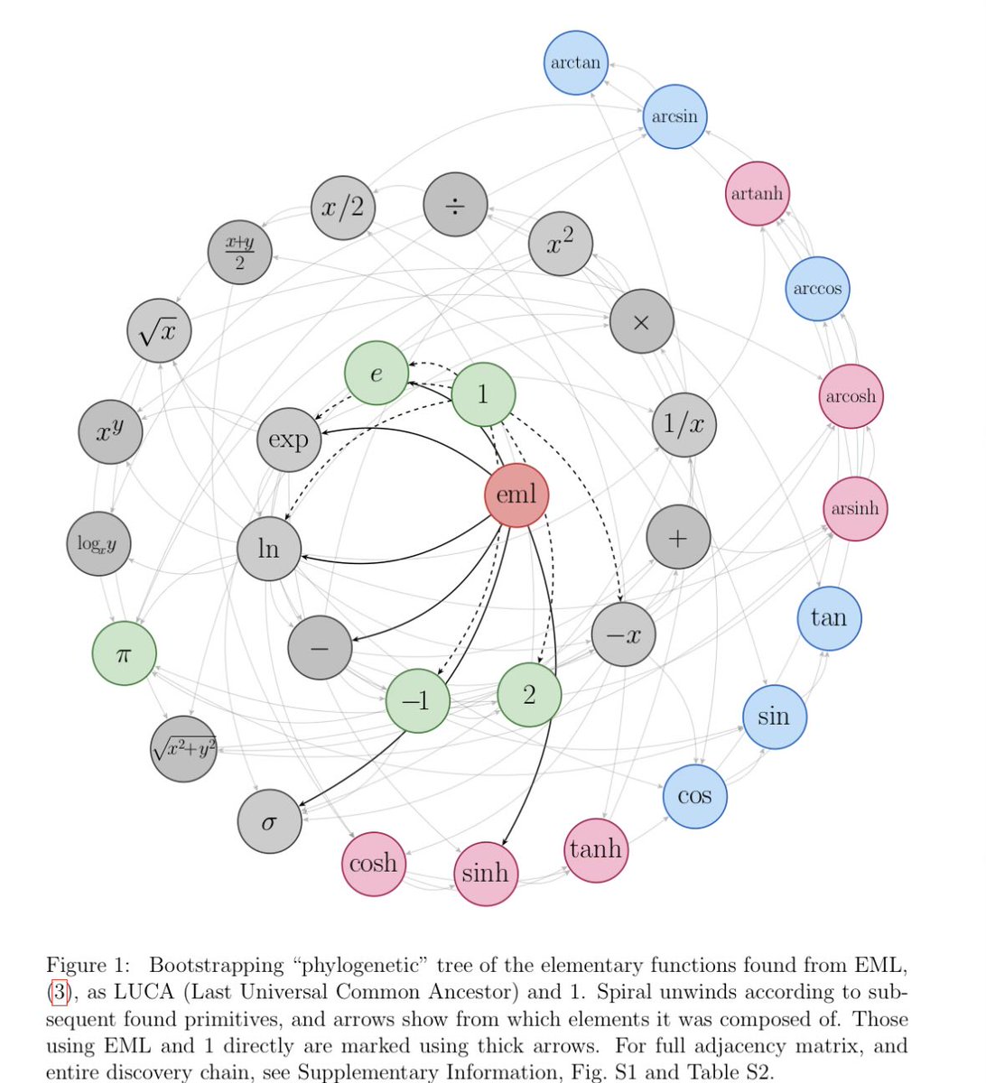
Polski naukowiec napisał ciekawą pracę - i nie bójmy się nazwać jej przełomową. Przez setki lat matematyka miała dziesiątki “podstawowych” funkcji jak sinus, cosinus, logarytm, pierwiastek, eksponenta. Znacie to ze szkoły. Wiadomo o co chodzi. Fizyk z Uniwersytetu Jagiellońskiego właśnie pokazał, że to wszystko jeden operator: E(x, y) = exp(x) - ln(y), oraz 1.

Sin, cos, π - wszystko z tego pięknie wynika, wystarczy odpowiednio zagnieździć. Natura ukryła najprostszy możliwy zapis rzeczywistości. I znaleźliśmy go przez przypadek. Całość jest piękna i wspaniała, a słowo „przełomowe” nie stanowi tu marketingowego buzzworda.

Przykładowo zamiast pisać π czy 3.14 można teraz elegancko E(E(E(1,E(E(1,E(1,E(E(1,E(E(1,E(E(1,E(1,E(E(1,1),1))),1)),E(E(E(E(E(1,E(E(1,E(1,E(E(1,E(E(E(1,E(E(1,E(1,E(E(1,1),1))),1)),E(E(1,E(E(1,E(E(1,E(E(1,1),1)),E(E(E(1,E(E(1,E(1,E(E(1,1),1))),1)),E(1,1)),1))),1)),1)),1)),1))),1)),E(E(E(1,E(E(1,E(1,E(E(1,1),1))),1)),E(E(1,E(E(1,E(1,E(E(1,E(E(1,E(E(1,E(1,E(E(1,1),1))),1)),E(1,1))),1))),1)),1)),1)),1),1),1))),1))),1)),E(E(E(1,E(E(1,E(1,E(E(1,1),1))),1)),E(E(1,E(E(1,E(1,E(E(1,E(E(1,E(E(1,E(1,E(E(1,1),1))),1)),E(1,1))),1))),1)),1)),1)),1)

[Curious | Macro Lens @CuriousMacroX]

Built this to track regime shifts
Sharing it below 👇

[Piotr Pomorski @PtrPomorski]

I dived deeper into MPC in my PhD but in terms of its use in multiperiod portfolio optimization. More on the subject can be read here (probably the best source): https://t.co/ohVCsr05lc

There is also a related python package: https://t.co/md4PWHgIN6. Have fun!

[Quant Beckman @quantbeckman]

It looks like ListFold-exp still needs more investigation, but it’s pretty interesting

[darkzodchi @zodchiii]

https://t.co/SRiKPtZufQ

[Piotr Pomorski @PtrPomorski]

Reminder:
- LR is mostly about L1 (lasso) or L2 (ridge) penalty
- Naive Bayes is alpha
- Decision tree nobody uses as a standalone algorithm but needs to be learnt how it works
- Random forest is all about max depth, no. of estimators, max features (cannot be all of them), min. samples split and leaf
- GBT is about using xgboost/catboost/lightgbm and focusing on the same as above + learning rate, alpha/lambda, no. of leaves, subsample/col. sample by tree, and boosting type if applicable
- PCA is all about leaving it alone for time series unless you roll / use it for research. PLS is good though. Types of PCA and when to use it:
-> linear for assuming linear relationships between features
-> kernel for nonlinear relationships between features -> incremental if you have tons of features and samples, and want to run PCA fast
-> robust PCA when you have outliers
- If we talk about PCA, one can mention ICA if you want statistically independent features rather than uncorrelated ones
- kNN is sometimes used; k-means is useful where obviously no. of clusters matter the most
- Support vector machine when nothing works and you're just curious if this one works. Relies on C and kernel, for capturing linear or nonlinear relationships
- NNs params is a story for another post, since these depend on types of NNs. But remember NN layer -> normalisation layer -> dropout layer. Sometimes you see activation layer between normalisation and dropout or even later; this depends if you want flexibility in terms of when to put it or you just drop it and add activation param inside the NN layer.

[Totozy Kely @T0t0zy]

@UncleBillz Should I be worried ? Should I read the terms before too late?

[gemchanger @gemchange_ltd]

https://t.co/bVArkKPyv1

[Piotr Pomorski @PtrPomorski]

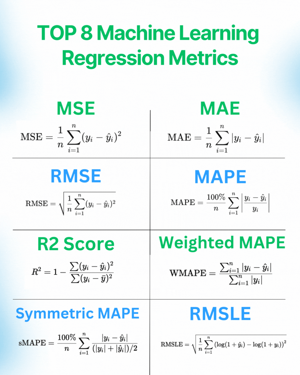
Reminder:
- MSE you use when you don’t have outliers
- RMSE you use when you want to interpret the above better
- MAE you use when you have positive/zero/negative values and outliers
- MAPE you use when you only have positive values and emphasize interpretability
- RMSLE you use for positive values with nonnormal distribution
- wMAPE you use when you want MAPE but have large vs small values
- sMAPE you use when you want MAPE but have zero/negative values
- R2 you use because your boss only knows this one

[Goshawk Trades @GoshawkTrades]

https://t.co/zY22h11YCE

[Piotr Pomorski @PtrPomorski]

Going deep https://t.co/8aQsi4vJXJ

[Roan @RohOnChain]

https://t.co/mzc1xbkxtQ