When matter meets its mirror, both vanish—and pure energy is born.
An electron and positron collide. Their rest masses disappear completely. What remains is two gamma rays racing outward, the exact conversion written as e⁻ + e⁺ → γ + γ. Nothing is lost; mass has simply changed form.
Scale that up to a proton and antiproton. Their quarks and antiquarks cancel, releasing a spray of new particles—pions, muons, photons, neutrinos—each carrying a share of the original mass-energy. The process is never the same twice.
E = mc² is not a slogan. It is the bookkeeping of the universe: every gram of matter holds the energy of a city, waiting only for its opposite to set it free.
📚 Algebra is more than formulas, it's a language that helps us describe patterns, solve problems, and understand the world. From Pascal’s Triangle to the quadratic equation, these mathematical essentials are the foundation of science, engineering, and data analysis. 🔢✨
The retina is a computer that throws away almost everything.
Raw light hits ~120 million photoreceptors. Through bipolar and ganglion layers it is filtered for contrast, edges, and motion, emerging as ~1 million optic-nerve fibers, a 100× compression performed entirely in analog.
Cameras still digitize every pixel, store it, then ship the flood to a distant processor. In-sensor chips place multi-layer register arrays at the photoreceptors themselves, computing the same features before any data leaves the chip.
The bandwidth problem was solved by biology long before we wrote the first line of code.
Paper stops alpha, aluminium stops beta, lead stops gamma and X-rays, water stops neutrons.
Alpha particles are helium nuclei that dump all their energy in the first few micrometres of matter. Beta particles are fast electrons that travel farther before they slow. Gamma rays and X-rays are photons that lose energy only through rare interactions, so only dense metal finally absorbs them. Neutrons carry no charge, so they ignore electric fields and need light nuclei in water or concrete to scatter and slow.
Shielding works because each particle asks matter a different question.
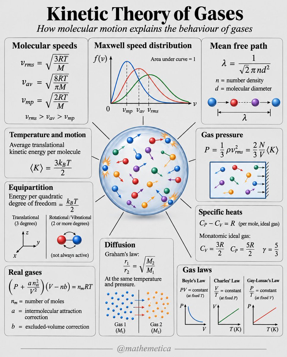
Every gas is a swarm of unseen collisions that somehow obey clean mathematical order.
Molecular speeds sort themselves into a precise hierarchy: the root-mean-square always outruns the average, which always outruns the most probable, all scaling with the square root of temperature over molar mass. The Maxwell distribution simply encodes that hierarchy so the area under the curve is always one.
The same microscopic bookkeeping yields the ideal-gas laws, specific heats, mean free path, and even Graham’s effusion ratio, all without ever watching a single molecule.
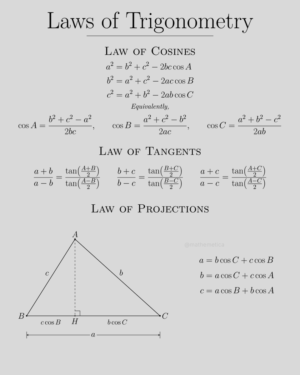
Triangles remember their angles through the sides.
The Law of Cosines generalizes Pythagoras: a² = b² + c² − 2bc cos A. When the angle is 90°, the cosine term vanishes and the familiar square relation remains. The rearranged form isolates each cosine so any side or angle can be recovered from the other three pieces.
The Law of Tangents pairs sums and differences: (a + b)/(a − b) = tan((A + B)/2) / tan((A − B)/2). It converts the awkward contrast of two sides into a clean ratio of half-angle tangents.
The projection formulas close the circle. Side a is exactly the sum of the adjacent sides projected onto it: a = b cos C + c cos B. Each side is the sum of the other two sides’ shadows.
Three laws, one triangle, every length and angle speaking the same language.
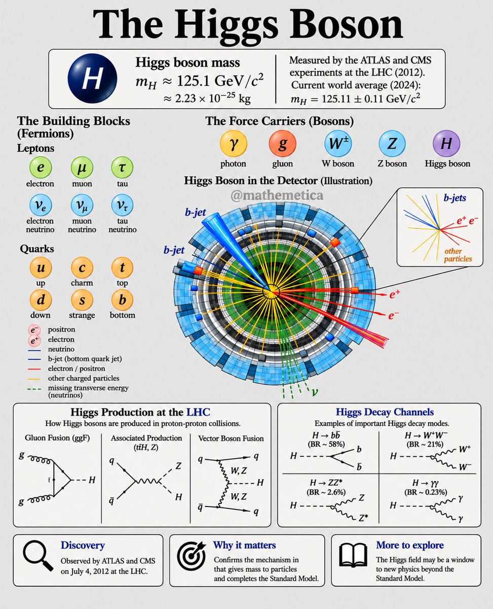
A single measured mass of 125.11 GeV/c² finished the Standard Model.
It equals 2.23 × 10⁻²⁵ kg. Produced mainly by gluon fusion in proton collisions, it decays with fixed branching ratios: ~58% to bb, ~21% to W⁺W⁻, ~2.6% to ZZ*, and only ~0.23% to γγ.
Those calculated probabilities matched the rare two-photon and four-lepton events recorded by ATLAS and CMS on 4 July 2012.
One number that closes the particle table and opens the next question.
Water’s phase diagram maps every stable state and the sharp boundaries that divide them.
At the triple point (0.01 °C, 0.006 atm) ice, liquid, and vapor coexist in equilibrium. Any small shift in temperature or pressure eliminates one phase.
The solid-liquid boundary slopes left because liquid water is denser than ice. That single geometric fact is why ice floats.
Past the critical point (374 °C, 218 atm) the liquid-gas distinction vanishes; only one fluid remains. A few lines and two special points capture the rare properties that make water essential to life.
partial derivatives are one of the most fundamental ideas in mathematics because almost nothing in the real world depends on just one variable. the temperature of a room depends on position and time. the motion of a robot depends on joint angles, velocities and external forces. the output of a neural network depends on millions of parameters. when multiple variables influence a system, the question becomes: how does changing one variable affect the output while everything else stays fixed? that’s exactly what a partial derivative measures. it isolates one relationship inside a much larger network of dependencies.
the interesting part is what happens when you start combining these derivatives. collect the partial derivatives of a scalar function and you get a gradient, which points toward the direction of steepest increase. organize the derivatives of multiple outputs with respect to multiple inputs and you get a jacobian, which describes how small changes propagate through a system. differentiate again and you begin describing curvature through second derivatives and the hessian. the chain rule connects these relationships across multiple functions, while the total differential tells you how their combined changes affect the output. these aren’t separate mathematical tricks. they’re different ways of organizing information about how a system responds to change.
this is why partial derivatives appear everywhere in modern engineering. backpropagation uses them to calculate how neural network parameters influence a loss function. robotics uses them to understand how joint movements affect the position of an end effector. fluid dynamics uses them to describe how velocity, pressure and temperature vary through space and time. control theory uses them to linearize nonlinear systems around operating points. the deeper idea is that engineering is fundamentally about understanding dependencies. once you can mathematically describe how one variable influences another, you can begin predicting, optimizing and controlling the entire system.
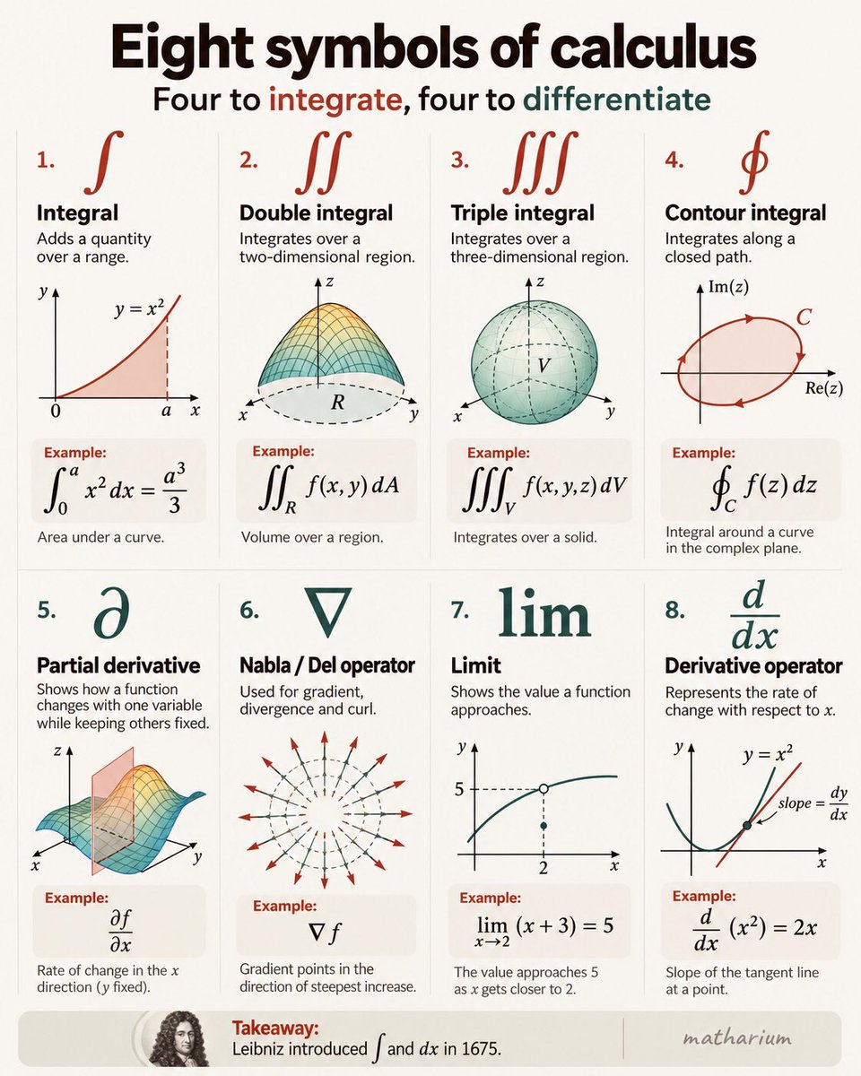
Eight symbols carry most of calculus. Four integrate: ∫ over an interval, ∬ over a region, ∭ over a volume, ∮ around a closed path. Four describe change: ∂, ∇, lim and d/dx.
∫₀ᵃ x² dx = a³/3 is the area under a parabola, ∂f/∂x changes x with other variables fixed, ∇f points uphill in the steepest direction, and d/dx (x²) = 2x is the slope of the tangent.
The symbols came from different people: Leibniz introduced ∫ and dx in 1675, ∂ was revived by Jacobi, ∇ came from Hamilton and lim from Lhuilier in 1786.
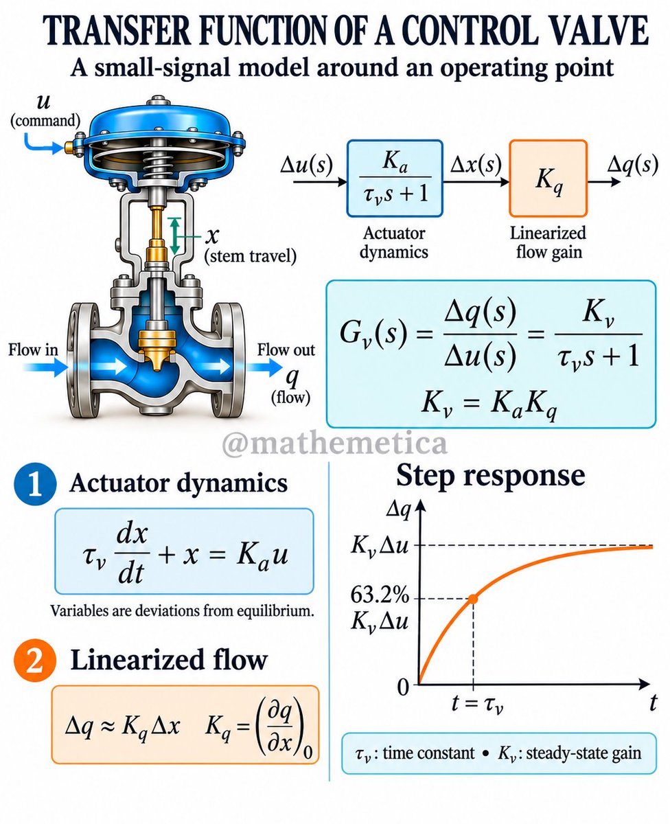
Every control valve is a first-order system around its operating point.
Stem travel obeys the lag τv dx/dt + x = Ka u. Flow then linearizes as Δq ≈ Kq Δx, with Kq equal to the local partial derivative of flow with respect to stem position.
Their product yields the clean transfer function Gv(s) = Kv / (τv s + 1), Kv = Ka Kq. A unit step therefore reaches 63.2% of its final value in exactly one time constant.
Small deviations convert messy valve physics into a single predictable exponential.
Why does nearly every noisy measurement in science and engineering, from height to sensor error, collapse into the same bell curve?
The normal distribution is the shape that appears whenever many small independent random influences add together. Its peak sits at the mean and it falls off symmetrically; about 68% of the mass lies within one standard deviation, 95% within two, and 99.7% within three.
Engineers use this to set quality-control limits that catch almost every defect, while machine-learning models treat residual noise as Gaussian so gradient updates stay well-behaved.