Ihsan

Mathematics Student

[Juanlu_CabanillasGar @JuanluCaba_Unex]

Think of a signal as a piece of music.
🎼 The Fourier Transform tells you which notes are being played.
🎻 The Laplace Transform tells you not only the notes, but also whether the music is fading away, growing louder, or becoming unstable.
#Engineering #Mathematics

[Math Hub @mathhub_vn]

Functions to Derivatives to Integrals

[Cosmos Archive @cosmosarcive]

A plane in 3D can be described in two surprisingly compact ways.

The vector form, n · (r − r₀) = 0, says that the displacement from a known point on the plane is perpendicular to the normal vector. Expand that dot product and you get the scalar form:

a(x − x₀) + b(y − y₀) + c(z − z₀) = 0

The key idea: the coefficients a, b, and c are not arbitrary. Together, they define the plane’s normal direction.

[Antonio Lupetti @antoniolupetti]

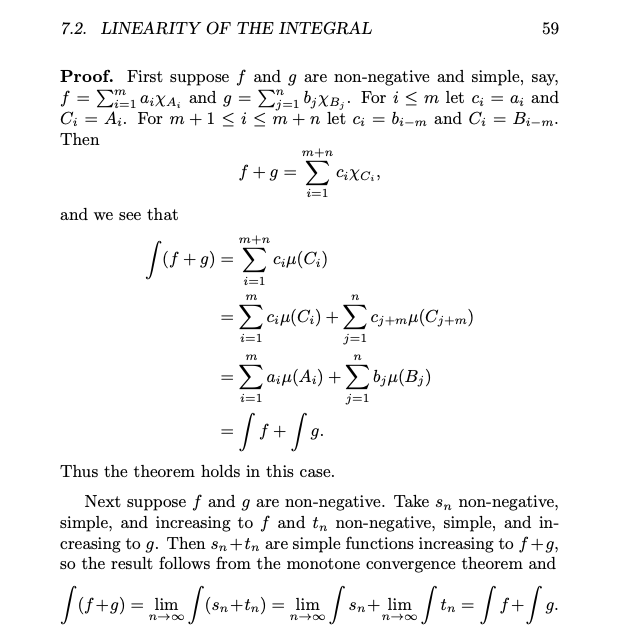
"Real Analysis" is an interesting set of free lecture notes for anyone who wants to move from introductory calculus to a more rigorous study of real analysis.

The notes cover measure theory, measurable functions, Lebesgue integration, Lp spaces, differentiation, Fourier analysis, and several other fundamental topics, with definitions, theorems, proofs, examples, and exercises.

I think these notes are a useful resource both for university students studying real analysis and for anyone looking for a solid reference to review these topics.

https://t.co/1uHshrsTWY

[Frank Nielsen @FrnkNlsn]

Ecosystem of Bregman divergences:

Fundamental convex duality yields many other dualities tied to BDs like:

- Bregman divergences ↔ exponential families
- Bregman divergences ↔ quasi-arithmetic centers
- Bregman divergences ↔ Hessian manifolds

https://t.co/5dfarHrOdN

[Python Developer @PythonDvz]

Patterns in Python with Examples

[SolvingForZ @SolvingForZ]

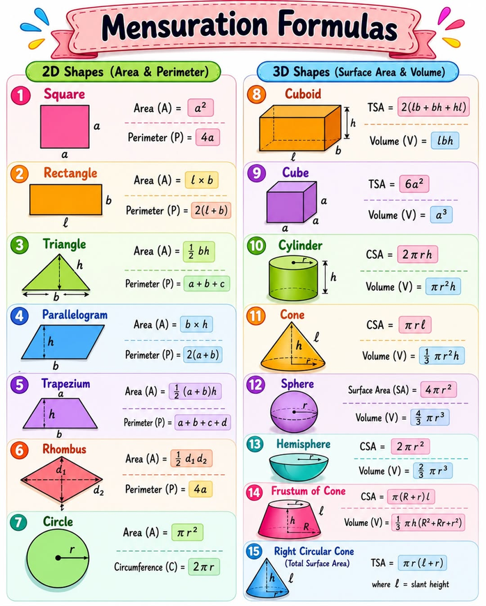
📏 Mensuration becomes easy when formulas are organised visually ✨

From 2D Shapes → Area & Perimeter to 3D Shapes → Surface Area & Volume, this cheat sheet covers the formulas students use again and again in exams 📚🔥

Don’t memorise blindly — understand the shape, remember the formula, solve faster. 🚀

💾 Save this for quick revision
📤 Share with your study partner

[SKG @sonukg4india]

🎯

[The Scientific Lens @LensScientific]

My favorite is the Dirac equation. Which one is yours?

[Math Hub @mathhub_vn]

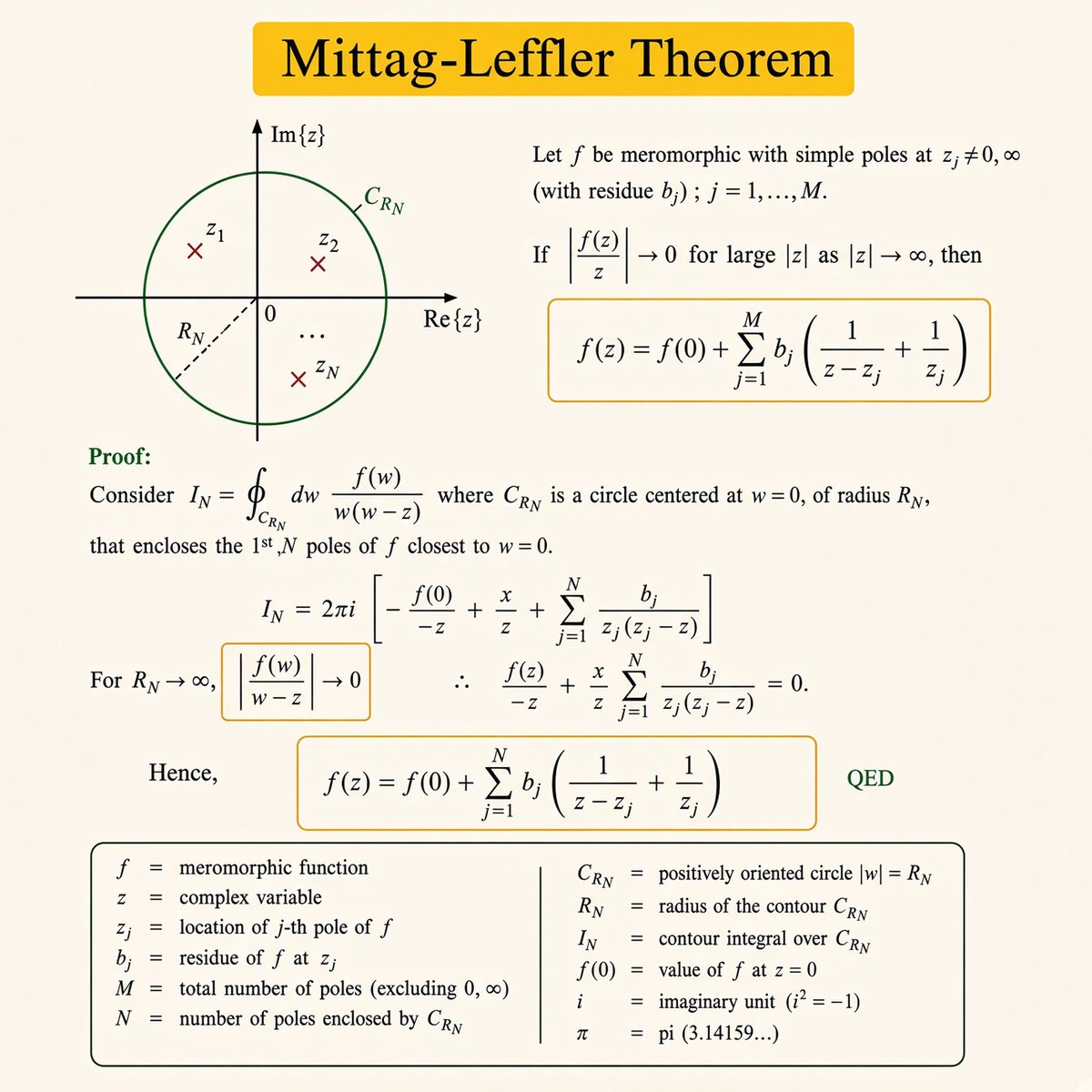
Mittag-Leffler Theorem - What if you could completely rebuild a function just by knowing where it fails and one number at each failure point? This sounds impossible. Yet this is what the Mittag-Leffler Theorem guarantees. It is one of the most impressive results in mathematics.

To grasp it, you need to explore complex numbers. Regular numbers exist on a line that stretches from negative infinity to positive infinity. Complex numbers break this one-dimensional limit and expand into a two-dimensional plane. Each complex number has a real part that moves horizontally and an imaginary part that moves vertically. Together, they fill an entire infinite plane rather than just a line. This expansion into two dimensions gives complex numbers unique properties that regular numbers lack and allows for remarkable mathematical results, including this theorem.

The theorem focuses on a special group of functions called meromorphic functions. Imagine a vast, smooth landscape extending infinitely in all directions. A meromorphic function is like that landscape but has infinitely tall, sharp spikes protruding from it. Everywhere except for the spikes, the landscape is smooth and predictable. Only at the spikes, known as poles, does the function become infinite and undefined. The poles are isolated, meaning each spike stands alone with clear space around it. Common examples include the tangent function, which spikes to infinity where the cosine equals zero, and any fraction with a denominator of zero.

Now, here is the magic. At each pole, there's an important number called the residue. The residue captures the essence of each spike how strongly the function blows up there, in what direction, and with what intensity. It serves as the defining feature of each singularity, a single complex number that identifies each breakdown point. The theorem states something remarkable. If you know where every pole is located, the residue at each pole, and the single value of the function at the origin, you can fully reconstruct the entire function everywhere. Not just approximately, but exactly. Every point across the infinite plane can be determined from this minimal local information.

The reconstruction works by summing contributions from all the poles at once. Each pole adds its own component to the total a term that spikes to infinity right at that pole's location, reflecting how the original function behaves there, then fading smoothly elsewhere. The residue at each pole determines the strength of its contribution. By combining the contributions from all the poles and including the value at the origin, you get the complete function perfectly rebuilt at every point from its singularities...

[Mathematica @mathemetica]

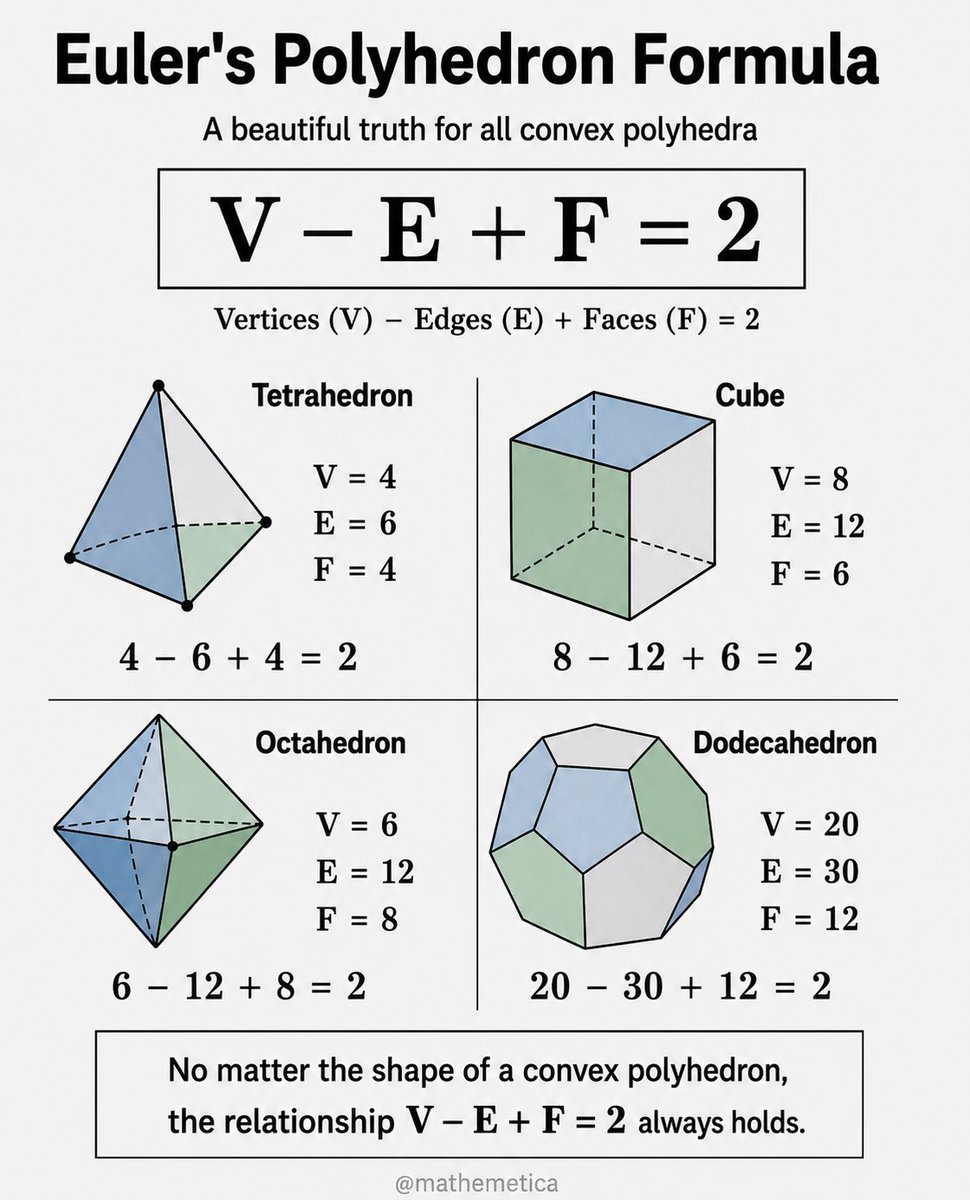
V − E + F = 2.

Whatever convex polyhedron one examines, the count of vertices minus edges plus faces returns the same integer.

A tetrahedron and a dodecahedron share almost no geometric resemblance, yet both produce exactly two. Face shapes and angles may vary freely; the underlying type of the surface cannot.

Euler first recorded the relation in 1750. The constant two is the Euler characteristic of the sphere, unchanged by any continuous deformation that neither tears nor punctures the surface.

[Math Magician @MathMagicianY]

Mathematical Symbols 🔢📐

[Matheorems @matheorems]

A messy rational function is almost always a sum of simpler pieces hiding in its factors.

P(x)/Q(x) = Σ Aᵢ / (x − aᵢ)^{nᵢ}

Distinct linear factors split as A/(x−a) + B/(x−b). A double root needs both 1/(x−a) and 1/(x−a)². Mixed factors simply add every required term.

This is how we invert Laplace transforms, expose the natural modes of circuits and control systems, and integrate rational functions by hand.
Each distinct factor contributes its own simple structure.

[Ihsan @ihsanmaths]

#mathematics #science #calculus

[Matheorems @matheorems]

An infinite bell curve hides a circle.

The volume under z = e^{-(x² + y²)} across the entire plane equals π.

In polar coordinates the integral separates:
∫₀^{2π} ∫₀^∞ e^{-r²} r dr dθ = 2π · ½ = π
This identity underpins the normal distribution, the heat equation, quantum ground states, and the Gaussians that shape modern machine learning.

Infinity can be finite when symmetry is complete.

[The Scientific Lens @LensScientific]

In 1736, Euler’s Seven Bridges of Königsberg problem showed that connectivity can matter more than geometry. It became a starting point for graph theory and an early step toward topology.

Topology asks: what stays the same when a shape is stretched or deformed? A sphere can become an ellipsoid. A solid torus can become a solid mug. But a sphere cannot become a torus without changing its topology.

[SKG @sonukg4india]

The figure of mathematics

[The Scientific Lens @LensScientific]

Gradient, Jacobian, and Hessian are three ways of describing how functions change.

[The Scientific Lens @LensScientific]

A metric tensor is the mathematical rule that tells us how distances and angles are measured in a space.
In ordinary Euclidean space, the Pythagorean theorem gives ds² = dx² + dy² + dz²
On a curved manifold, that rule becomes ds² = gᵢⱼ dxⁱ dxʲ

The components gᵢⱼ determine how the coordinates contribute to local lengths and angles. They form a symmetric matrix, and from the metric, the geometry of the space can be described. Riemann’s insight was that geometry does not need to begin with a fixed notion of distance. The metric itself can define what “distance” means.