Tambet Matiisen

[Zhuokai Zhao @zhuokaiz]

The best paper I’ve read on world models this month solved collapse with a statistics theorem from 1936.

LeWorldModel (LeWM) has been getting a lot of attention, and rightfully so. Several great reviews like the one by @ID_AA_Carmack have already covered the architecture and implementation details.

However, I want to share personally why I think this paper matters a lot for the broader world model landscape, and what it tells us about the role of inductive biases in representation learning.

JEPA-based world models always have this beautiful idea: encode observations into compact latent spaces, predict dynamics there, while skipping pixel-level generation entirely.

But in practice, they often collapse: the encoder learns to map everything to nearly the same vector, prediction loss goes to zero, and the representation loses all meaningful structure.

This has been one of the central headaches of JEPA training from the beginning.

The field’s response has been to pile on tricks to prevent collapse: keeping a second copy of the encoder that updates more slowly than the main one (exponential moving average) and blocking gradients from flowing through it; freezing pre-trained backbones entirely; or using multi-term losses like VICReg with several coefficients to tune.

These ideas work, but their theoretical grounding is still limited — we don’t really have a clean objective-level understanding of what EMA + stop-gradient is minimizing. We just know it often avoids collapse.

LeWM’s fix is extremely simple: it forces the latent embeddings toward an isotropic Gaussian.

Because if your embeddings match an isotropic Gaussian, they cannot all collapse to the same point, so trivial collapse becomes incompatible with the objective.

The clever part is how they enforce this, since testing Gaussianity in high-dimensional space is hard.

Classical normality tests are designed for 1D data and don't scale well to high dimensions.

But the Cramér-Wold theorem (1936) offers an elegant workaround: a multivariate distribution is Gaussian if and only if all its 1D linear projections are Gaussian.

This means you can sample random directions, project your embeddings onto them, run a cheap univariate normality test (Epps-Pulley) on each projection, and average the statistics as your regularization loss.

They call this SIGReg.

The resulting training objective is just two terms:
(a). a standard MSE loss between predicted and actual next-step embeddings, plus
(b). λ-weighted SIGReg on the embeddings to keep them Gaussian.

So essentially, SIGReg leaves you with only one effective hyper-parameter to tune (λ), with no EMA, no stop-gradient, and no pre-trained encoder. And all parameters are trained end-to-end.

What I like the most / find most interesting

1. The inductive bias argument
PLDM, the previous end-to-end JEPA, tries to prevent collapse by stacking multiple regularization terms (variance, covariance, temporal smoothness, etc.) without a single unifying principle. Each term fights collapse from a different angle, so it ends up tuning multiple coefficients to balance them, requiring a much more expensive hyper-parameter search.

LeWM takes the opposite approach. SIGReg enforces one well-chosen inductive bias: that good latent representations should follow an isotropic Gaussian distribution, so there is less need to separately enforce variance, decorrelate features, or smooth trajectories. Because in principle, a collapsed representation where everything maps to one point is obviously not Gaussian.

And the results back this up: LeWM hits 96% success on Push-T vs. PLDM’s 78%, with dramatically lower training variance across seeds.

2. The paper also reports where LeWM falls short
LeWM doesn’t uniformly dominate.

It wins clearly on Push-T (96% vs DINO-WM’s 92%) and Reacher (86% vs 78-79%), but underperforms on Two-Room (87% vs ~100%) and OGBench-Cube (74% vs DINO-WM’s 86%).

But the authors explain why: in very low-dimensional environments, forcing a high-dimensional isotropic Gaussian prior may over-constrain the representation. In visually complex 3D scenes, end-to-end encoder training is still harder than leveraging DINOv2’s 124M-image pre-training.

3. The planning efficiency story
Because LeWM’s encoder outputs ~200-dim embeddings vs DINO-WM’s ~40,000 tokens, planning is ~48× faster (0.98s vs 47s for a full plan).

Under a fixed compute budget, this gap becomes dramatic: 90% success on Push-T vs. DINO-WM’s 13%. (If you care about deploying world models with limited compute, this matters a lot.)

4. Emergent temporal straightening
This is the most interesting result.

When you encode a sequence of observations into latent space, you get a sequence of embedding vectors.

Between consecutive time steps, you can compute the change vector (just z_{t+1} minus z_t), and then check whether consecutive change vectors point in similar directions by computing their cosine similarity.

High cosine similarity indicates the trajectory traces a near-straight line in latent space, meaning that the representation evolves smoothly and predictably over time, much like how a physically plausible motion follows a smooth path in the real world.

Without any explicit temporal regularization, LeWM’s latent trajectories become increasingly straight over training.

PLDM explicitly optimizes for temporal smoothness with a dedicated loss term, yet LeWM achieves higher straightness as an emergent property of the Gaussian constraint.

This actually connects to the temporal straightening hypothesis from neuroscience, where they found that biological visual systems also tend to straighten temporal representations of natural videos. What's interesting here is that LeWM achieves this without ever explicitly asking for it — the Gaussian distributional prior alone seems to be enough to induce this kind of temporal structure.

Zooming out: what this means for the world model landscape

There’s a growing tension in the world model space between two philosophies:

1. The foundation-model-first approach:
Freeze a massive pre-trained vision encoder (DINOv2, CLIP), and only train a small predictor on top to learn the dynamics. This gives strong representations out of the box, but the system is fundamentally bounded by what the encoder learned during pre-training. DINO-WM is the representative work here.

2. The end-to-end-from-scratch approach:
train encoder and predictor jointly, taking raw pixels as input but predicting in latent space. Maximum expressivity, but collapse has been a nightmare and has required significant engineering to handle. PLDM tried this but struggled with training instability, which is exactly the problem LeWM addresses with SIGReg.

What LeWM demonstrates is that the end-to-end approach is viable — and may be preferable for specific tasks.

A 15M-parameter model trained on a single GPU for a few hours can match or beat a system built on DINOv2, which was pre-trained on 124M images across massive compute.

The key insight here is that when your task is predicting how an environment evolves over time, task-specific representations learned end-to-end can outperform generic pre-trained features, as long as you solve the collapse problem cleanly.

I think this is worth paying attention to, especially as the field increasingly defaults to freezing large pre-trained backbones for everything.

That works well for general-purpose tasks, but for something as specific as learning environment dynamics from interaction data, the right end-to-end training objective can do more with far less.

15M params. One effective hyper-parameter. Single GPU. A 90-year-old theorem.

Sometimes simplicity is the breakthrough.

[Igor Babuschkin @ibab]

Took a break from Claude coding to write a little story
https://t.co/ZtuRzJZ4RM

[Arman Hezarkhani @ArmanHezarkhani]

https://t.co/HUDx91vIIh

[Tambet Matiisen @tambetm]

I just realized what the future of software is going to look like - like Claude Code. A lot nice-to-have bling alongside the core functionality. It used to be maintenance nightmare, but now it’s almost free.

[outside five sigma @jwt0625]

your finger press over ~10 ms closes a switch in a keyboard matrix, during which ~10¹³ electrons flow through pull-up resistors and scan circuitry. Firmware encodes the event, and a microcontroller emits a USB or Bluetooth HID report of a few dozen bytes.

the OS services an interrupt in a few us, maps scan codes to characters, and updates 10²~10³ bytes of state in DRAM, stored as charge from ~10⁸ electrons on capacitors refreshed every ~60 ms.

your browser constructs an HTTPS request of 1~5 kB, which the TCP/IP stack segments into ~1.5 kB payloads matched to the Ethernet MTU. These drive a network interface with SerDes operating at a few GHz, shoving 10⁶~10⁸ electrons per bit.

electrical signals propagate a few cm across copper traces, then drive optical transceivers where electrons jump a semiconductor bandgap to emit 10⁶~10⁸ photons per bit at telecom wavelengths. These photons traverse access, metro, and backbone networks, undergoing a dozen electrical <-> optical conversions at endpoints and regeneration sites.

these photons might further go through hundreds to thousands of kilometers of fiber, amplified every ~100 km by erbium-doped fiber amplifiers via stimulated emission, wavelength-routed by ROADMs, might even bounce off google's MEMS optical circuit switches a few times, and eventually reconverted to electrons by photodiodes at termination and routing boundaries.

at the data center, packets are reassembled and delivered to inference servers where GPUs perform matrix multiplications involving ~10¹² model parameters over milliseconds, with transistors toggling at 10¹⁶~10¹⁷ times per second.

those parameters were produced earlier by training runs lasting weeks to months, using ~10⁴ accelerators drawing who knows how many megawatts of power, shoving 10³⁰~10³³ electrons through transistor channels for the 10²³~10²⁵ floating-point operations.

the inference result is serialized into kilobytes of data and transmitted back through the same chain, again undergoing repeated electrical - optical - electrical conversions across access, metro, and backbone networks.

back on your phone or laptop or whatever, the browser parses the response, updates layout and rendering structures, and issues GPU draw calls that write millions of pixels per frame into a framebuffer at 60~120 Hz.

display interfaces stream multiple gigabits per second to an OLED or microLED panel, where the pixels emit roughly 10⁸~10¹¹ visible photons per frame, driven by ~microamp currents over ~microsecond switching intervals.

those photons traverse a few meters in nanoseconds, absorbed by your retinal photoreceptors, transduced into electrochemical signals, and interpreted by a ~20 W biological neural system.

end-to-end, you have astronomical numbers of highly coordinated electrons and photons, and dozens of conversions between them (ofc not including training), for a single thought from the little intelligence to appear on a screen and read by you.

[Tambet Matiisen @tambetm]

@wzihanw If you have a perfect value function, the credit assignment becomes trivial - the action that led to sudden jump in current state value must have been valuable action.

[Tambet Matiisen @tambetm]

@f14bertolotti There is quite a number of works exploring this idea:
https://t.co/gOG5PwWoy3
https://t.co/Ac137WCuFo
https://t.co/NJp5zjbGh1
The latter two do not use backpropagation through world model though…

[will depue @willdepue]

you tend to hear this a lot from people outside or new to ML, and I often point to a talk Ilya gave a few years back:

1) think of any decent deep neural net that has enough memory and sequential ops as just a big parallel computer

2) training this neural net is doing search over computer programs that maximize your objective

3)unless you have some large bottleneck (and given you can successfully optimize this system) you’ll find that these parallel computers are highly robust to architectural changes.

4) this is because computers are great at simulating each other. your new architecture can usually be straightforwardly simulated ‘inside’ your old architecture.

5) it’s not that architecture doesn’t matter, but it mostly matters with respect to (1) fundamental bottlenecks in this parallel computer (2) modifications that make models easier to optimize, since this argument only holds if your optimization is good (3) compute efficiency/system efficiency wins that make learning easier or faster.

6) it’s quite possible that new architectures will lead to breakthroughs in machine learning, but we should first start with bottlenecks, not naturalist intuitions about the ‘form’ of AI should take. until you understand this it seems surprising that small models trained longer are better than undertrained big models, that depth and width are surprisingly interchangeable, that talking to a model with an MoE or sparse attention or linear attention is approximately the same iso evals.

[Yoonho Lee @yoonholeee]

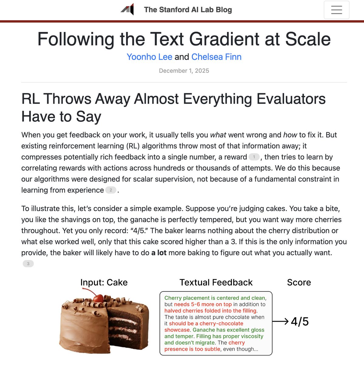
Following the Text Gradient at Scale

We wrote a @StanfordAILab blog post about the limitations of RL methods that learn solely from scalar rewards + a new method that addresses this

Blog: https://t.co/rJ1IcBKDoR
Paper: https://t.co/75pHtElyk3

[Tambet Matiisen @tambetm]

@alexgkendall This is cool, but unpredictable, which of these behaviors emerge from end-to-end training and to which situations they generalize. How can we make generalization more predictable?

[Tambet Matiisen @tambetm]

@___Harald___ @comma_ai How I think this slide should be read:
- 80% autonomy (just highways) takes 5W
- 99% autonomy (supervised) takes 170W
- 99.99% autonomy (unsupervised) takes 1500W

[Tambet Matiisen @tambetm]

@___Harald___ @comma_ai Don’t take the prize literally. What I mean is that 80% of something takes 20% of the effort. But consumers usually want 100% of the product. And the last 20% will take 80% of your effort. Or watts, if you prefer. Each 9 will be just as hard as the previous 9.

[Tambet Matiisen @tambetm]

@___Harald___ @comma_ai This is not unique to comma, other strong ADAS companies are also struggling to make a leap to full self-driving. Take Mobileye.

[Tambet Matiisen @tambetm]

@___Harald___ @comma_ai While I admire comma’s desire to bootstrap themselves into self-driving business, there have not been any major improvements to autonomy capability for years. Producing shippable intermediaries seems to consume all the energy and not much is left for solving self-driving.

[Tambet Matiisen @tambetm]

@comma_ai Over 80% of the data is from the US, while previously it was ~ 50%. Why the data from the rest of the world is less emphasized? Does it mean that the new model will work worse in Europe?

[Tambet Matiisen @tambetm]

@karpathy That’s your learned credit assignment. The distributed reward basically acts as advantage in the policy gradient formula, increasing the probability of taken action. And it’s all nicely normalized, no need for advantage normalization.

[Tambet Matiisen @tambetm]

@karpathy But I can see that being pretty limiting. Probably makes sense to do couple of self-attention steps between all sequence states first. This allows the reward-inducing properties of the states to propagate to nearby (similar) states.