Wy

Focus on automation control
这短短的一生，我们最终都会失去；你不妨大胆一些，爱一个人，攀一座山，追一个梦。

[Mathematica @mathemetica]

Four equations that turned invisible forces into light.

Maxwell unified electricity and magnetism into a single framework. A changing electric field creates a magnetic field, and a changing magnetic field creates an electric field. Together they sustain each other, racing outward as electromagnetic waves at the speed of light.

Gauss’s laws fix the sources: charge produces electric field lines, while magnetic field lines never begin or end. Faraday and Ampère (with Maxwell’s correction) show how the fields continually generate one another.

From these four lines, radio, light, and the entire modern world quietly emerge.

[Historic Vids @historyinmemes]

“A tiger wearing a bell will starve.”

- Mongolian Proverb

This is a powerful Mongolian proverb that emphasizes the value of silence, patience, and discretion in achieving success. It reminds us that even the strongest and most capable individuals can undermine their own potential by revealing their intentions too soon.

Just as the sound of a bell warns a tiger’s prey of its approach, constantly announcing your ambitions can expose your plans to unnecessary attention, competition, and interference. True strength is not always displayed through words or recognition, but through quiet determination and deliberate action. The lesson is simple: move in silence, remain focused on your goals, and allow your accomplishments to speak louder than your promises.

[Mustafa. @oprydai]

study algebra. not as the art of finding x.

as the art of reasoning about things you do not know yet.

• variables → name the unknown and work with it anyway
• equations → state a constraint, then solve backward
• linear algebra → solve millions of equations at once
• groups → the mathematics of symmetry
• finite fields → the arithmetic behind encryption and error correction

> the word comes from al-khwarizmi's 9th-century book. so does "algorithm," from his name.
> boole turned logic into algebra in 1854. every digital circuit still runs on it.
> galois died at 20. his groups explain why no formula solves the quintic.
> a rubik's cube is a group with 43 quintillion elements.
> every qr code you scan repairs itself using finite field algebra.

arithmetic works with numbers. algebra works with structure.

learn to solve the pattern once, and you have solved every case of it.

[İçsel Güç @Icsel_Guc]

Machiavelli’ye göre iş yerinde ve kariyerde ayakta kalmanın 3 temel noktası:

[İçsel Güç @Icsel_Guc]

Kendi Gücüne Dayanmak

Başkalarının ordularına, sözlerine veya dostluklarına güvenerek yola çıkmamak; en güvenli kalenin kendi yetkinliğin ve hazırlığın olduğunu asla unutmamak.

Örneğin; sadece bir şirkete, bir unvana ya da başkalarının getireceği iş fırsatlarına bağımlı yaşamak büyük bir riskiktir.

Kendi beceri setini sürekli güncellemek, kendi sermayeni ve alternatif üretim kanallarını yaratmak gerçek bağımsızlıktır.

[Physics In History @PhysInHistory]

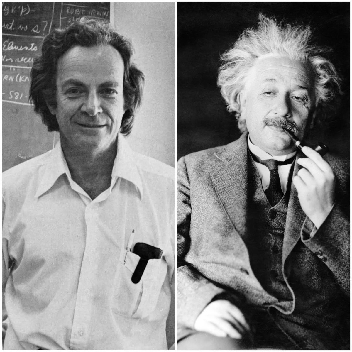
When Richard Feynman met Albert Einstein 💭

It was Feynman’s first encounter with Einstein. When the seminar finally started, Feynman’s hands were shaking, in the beginning, seeing all those great minds of the time. He would call them monster minds. But as he started with the seminar and dug deep down into the actual topic he was fearlessand couldn’t think of anything else except the topic he was explaining. He said,

“the moment I start to think about Physics, and have to concentrate on what I’m explaining, nothing else occupies my mind. I’m completelyimmune to being nervous.”

[Mustafa. @oprydai]

Study physics.

if you want to understand how reality works, this is not optional.

• mechanics → forces, motion, energy, momentum
• thermodynamics → heat, work, entropy, energy transfer
• electromagnetism → electricity, magnetism, circuits, fields
• waves & optics → oscillations, sound, light, interference
• quantum mechanics → matter and energy at microscopic scales

but don’t just memorize equations.

> derive them.
> understand the assumptions.
> solve problems.
> run simulations.
> build experiments.

physics connects mathematics to the physical world.

it’s the foundation of mechanical engineering, electronics, robotics, materials science, and much of modern technology.

learn the laws of nature. then learn how to engineer within them.

[Matheorems @matheorems]

Gradient, Divergence and Curl

Three vector fields, moving at the same time.

Gradient: phi = 1 - x^2 - 2y^2, so grad phi = (-2x, -4y). Every tracer flows uphill and crosses each contour at a right angle. The red probe climbs to the top, and its arrow shrinks to zero there, because the slope at a peak is zero.

Divergence: F = (x, y) pushes out of every point, div F = 1 + 1 = 2 (a source). Flip it to F = (-x, -y) and div F = -2 (a sink): the flux through the circle turns around.

Curl: F = (-y, x) turns everything around the centre, curl F = 1 - (-1) = 2, pointing out of the screen. A paddle wheel carried by the flow spins once per orbit. Reverse the field and the curl points into the screen, -2.

[Joruno @wsl8297]

你听过最有水平的一句话是什么？

[Matheorems @matheorems]

The Five Differential Operators of Physics

Five operators built from one symbol, nabla, all moving at once.

Divergence: div F = dFx/dx + dFy/dy + dFz/dz, the net flux out of a tiny closed surface (source or sink strength).

Gradient: grad phi = (dphi/dx, dphi/dy, dphi/dz) points to the steepest increase of phi, always at a right angle to the contour lines, and is longest where they are tightest.

Curl: curl F measures the spin of the field around a point. The vector stands on the axis of the whirl, and flips when the whirl reverses.

Laplacian: the sum of the second derivatives. On the bowl z = x^2 + y^2 the Laplacian is 4, so the average around any circle of radius r sits exactly r^2 above its centre.

D'Alembertian: box F = (1/c^2) d^2F/dt^2 - Laplacian F. A wave running at speed c makes it zero, which is why it appears in the wave equation and in relativity.

[Wy @BeWiseRobot]

@oprydai 👍👍👍

[Mustafa. @oprydai]

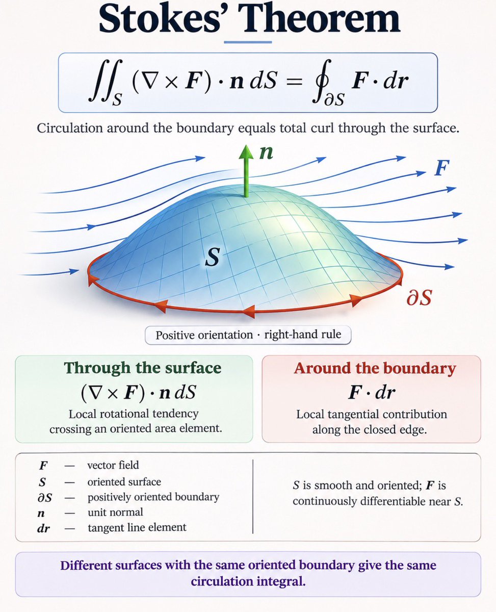
stokes’ theorem is one of those mathematical ideas that reveals how deeply local behavior is connected to global behavior. imagine a fluid flowing across a curved surface. at every tiny point, the fluid has some tendency to rotate, which we describe using curl. now imagine walking around the boundary of that surface and measuring how much the fluid flows along your path. stokes’ theorem tells us that these two seemingly different measurements are actually equal. the total rotational tendency accumulated across the surface is exactly the circulation measured around its boundary.

the intuition becomes clearer when you divide the surface into thousands of tiny patches. each patch has its own circulation along its edges. but when you add them together, the contributions along shared internal edges cancel because neighboring patches traverse those edges in opposite directions. what remains is only the circulation around the outer boundary. that’s the beautiful part. an integral over an entire two dimensional surface can be replaced by an integral around a one dimensional curve. the theorem doesn’t just simplify calculations. it exposes a fundamental relationship between what happens inside a region and what happens along its edge.

this is why stokes’ theorem appears throughout physics and engineering. in electromagnetism, it connects the circulation of electric and magnetic fields to their local curl, allowing maxwell’s equations to be expressed in integral and differential forms. in fluid mechanics, it relates vorticity distributed across a surface to circulation around its boundary. the deeper idea is that local interactions can accumulate into global effects, while internal contributions cancel and leave a measurable result at the boundary. once you recognize this pattern, you begin seeing the same mathematical structure in green’s theorem, the divergence theorem and the generalized stokes’ theorem. different dimensions, different geometries, but the same underlying principle: the behavior of a system’s interior is connected to the behavior of its boundary.

[Mustafa. @oprydai]

partial derivatives are one of the most fundamental ideas in mathematics because almost nothing in the real world depends on just one variable. the temperature of a room depends on position and time. the motion of a robot depends on joint angles, velocities and external forces. the output of a neural network depends on millions of parameters. when multiple variables influence a system, the question becomes: how does changing one variable affect the output while everything else stays fixed? that’s exactly what a partial derivative measures. it isolates one relationship inside a much larger network of dependencies.

the interesting part is what happens when you start combining these derivatives. collect the partial derivatives of a scalar function and you get a gradient, which points toward the direction of steepest increase. organize the derivatives of multiple outputs with respect to multiple inputs and you get a jacobian, which describes how small changes propagate through a system. differentiate again and you begin describing curvature through second derivatives and the hessian. the chain rule connects these relationships across multiple functions, while the total differential tells you how their combined changes affect the output. these aren’t separate mathematical tricks. they’re different ways of organizing information about how a system responds to change.

this is why partial derivatives appear everywhere in modern engineering. backpropagation uses them to calculate how neural network parameters influence a loss function. robotics uses them to understand how joint movements affect the position of an end effector. fluid dynamics uses them to describe how velocity, pressure and temperature vary through space and time. control theory uses them to linearize nonlinear systems around operating points. the deeper idea is that engineering is fundamentally about understanding dependencies. once you can mathematically describe how one variable influences another, you can begin predicting, optimizing and controlling the entire system.

[Reads with Ravi @readswithravi]

“Spend your money on the things money can buy. Spend your time on the things money can't buy.”

— Haruki Murakami

[Bitturing @Bitturing]

🚨提醒：你用 ChatGPT 和 Claude 写的东西，别人一眼就能看出来。

结构太整齐、语气太客套、打磨得太过头。这些都会暴露。

7 条提示词帮你改掉：

[Matheorems @matheorems]

Eight calculus symbols, all moving at once.

Integral: the area under y = x^2 sweeps up to a, and it equals a^3/3.

Double integral: the region R fills up with little squares dA, then again with finer ones.

Triple integral: the ellipsoid V fills up with little cubes dV, layer by layer, while it turns.

Contour integral: a point goes round the closed path C.
Partial derivative: cut the surface at a fixed y, and slide the tangent in the x direction. That slope is df/dx.

Nabla: the gradient arrows of f point outward.
Limit: the point gets closer and closer to (a, L), but the circle there stays open.

Derivative: a tangent line rolls along y = x^2, and its slope is always 2x.

[Physics In History @PhysInHistory]

A page from Einstein's 16-page manuscript, dated 1924, found by a student by accident at a university in the Netherlands.

[Math Files @Math_files]

On September 18, 1783, the 76-year-old Leonhard Euler spent his final day doing mathematics.

Almost blind, he gave a mathematics lesson to a grandchild, worked with chalk on the motion of rising balloons, and discussed the orbit of Uranus, a planet discovered just two years earlier.

Balloon flight was then a remarkable new development. Euler was investigating how high a balloon could rise and how its motion could be calculated.

Later that afternoon, he suffered a cerebral hemorrhage. He never recovered.

But there is an extraordinary detail.

The calculations left on Euler's slate were preserved. In 1784, the Paris Academy of Sciences published them in a paper identifying them as the calculations found after his death.

The work survives today as Euler's paper E579.

Even on his final day, one of history's most productive mathematicians was investigating a scientific problem that had only recently captured Europe's imagination.

[Mustafa. @oprydai]

gradient, jacobian, and hessian are three mathematical tools that describe how a system changes, but at different levels. the gradient tells you how a single output responds to changes in multiple inputs. imagine standing on a mountain and wanting to know which direction takes you uphill the fastest. that’s your gradient. the jacobian extends this idea to systems with multiple outputs. instead of one mountain, imagine a robotic arm where changing one joint angle affects the position of the end effector in several directions. the jacobian captures all those local relationships in one matrix. the hessian goes a level deeper. it describes how the gradient itself changes, revealing the curvature of the function.

the interesting part is how these concepts connect to optimization and robotics. gradient descent uses the gradient to determine which direction reduces an error or loss function. the jacobian tells a robot how small changes in joint angles translate into changes in position and orientation, making it fundamental to inverse kinematics, motion control and sensitivity analysis. the hessian describes the local curvature of an objective function, helping optimization algorithms distinguish flat regions from steep ones and understand how the best direction changes. first derivatives tell you how a system responds. second derivatives tell you how that response itself evolves.

what i find beautiful is that these aren’t three unrelated mathematical inventions. they’re different levels of the same idea: understanding dependencies between variables. the gradient describes local sensitivity for one output, the jacobian organizes sensitivities across many outputs, and the hessian captures how those sensitivities change for a scalar function. once you understand this structure, multivariable calculus becomes much more intuitive. robotics, machine learning, computer vision, physics and optimization all keep returning to the same fundamental question: if i change something in this system, what happens to everything else, and how does that relationship change as the system evolves?

[Mustafa. @oprydai]

tensor calculus is one of those subjects that completely changes how you understand geometry and physics. ordinary calculus tells you how quantities change, but tensor calculus goes a step further. it asks how quantities change when the coordinate system itself is changing, especially when you’re working on curved surfaces or spacetime. a vector might have different numerical components depending on how you describe it, but the physical quantity it represents remains the same. tensors give us a mathematical language to preserve that underlying structure regardless of the coordinates we choose.

the interesting part begins with the metric, which tells us how to measure distances and angles. then comes the connection, which tells us how to compare directions at neighboring points. on a curved surface, you cannot simply move a vector from one location to another and assume its direction remains unchanged. parallel transport gives us a rule for moving it, while the covariant derivative measures how a tensor changes after accounting for the changing geometry. once you understand these ideas, curvature stops being something you only visualize and becomes something you can calculate. this is the mathematical machinery that allows us to describe curved spaces consistently.

and this is where tensor calculus becomes fundamental to general relativity. einstein’s field equations connect the geometry of spacetime to the energy and momentum of matter. gravity is no longer treated simply as a force pulling objects toward one another. it becomes a consequence of the geometry through which objects move. the same mathematical ideas also appear in continuum mechanics, fluid dynamics, elasticity and differential geometry. what i find beautiful is that tensor calculus is really about separating physical reality from the coordinates we use to describe it. the equations may change their appearance, but the underlying relationships remain invariant. that’s one of the deepest principles in mathematics: a good description of reality should not depend on the perspective from which you observe it.