Neither @oswinso nor I could make it to ICLR this year, but our poster did make the trip 🤣✈️🇧🇷
Come by our poster today about #DAM (#Discrete#Adjoint#Matching)—a unifying AM for discrete generative models (e.g., dLLM) !!
🕒 3:15 PM – 5:45 PM
📍 Pavilion 3 P3 #1711
Adjoint Matching works great for fine-tuning diffusion models with reward gradients.
How about #AM for #diffusionLLMs with #nondifferentiable#rewards? Does "discrete adjoint" even exist ... and how? 🤔
📢 Introduce #DiscreteAdjointMatching (#DAM)—a unifying AM for discrete generative models, accepted to #ICLR2026 🇧🇷
Work done with my amazing intern @oswinso and @RickyTQChen, Brian, Chuchu 🙌
📰 https://t.co/v2CcenlkAT
At #NeurIPS from Dec 2 to Dec 7 in San Diego! Looking forward to catching up and meeting new friends.
Excited to chat about safety for robotics, constraint satisfaction in RL, and (stochastic) optimal control.
Feel free to DM me to grab coffee or have a chat!
Robots can plan, but rarely improvise. How do we move beyond pick-and-place to multi-object, improvisational manipulation without giving up completeness guarantees?
We introduce Shortcut Learning for Abstract Planning (SLAP), a new method that uses reinforcement learning (RL) to discover shortcuts in the planning graphs induced by task and motion planning (TAMP) skill libraries. It is a plug-and-play module that can be trained on top of existing planners to speed up execution through learned shortcuts.
(1/5)
Meet Casper👻, a friendly robot sidekick who shadows your day, decodes your intents on the fly, and lends a hand while you stay in control!
Instead of passively receiving commands, what if a robot actively sense what you need in the background, and step in when confident? (1/n)
@Almost_Sure Yeah, I was thinking about it from the perspective of using Feller’s test of explosion to show that it either hits zero in finite time or explodes to infinity, and that former happens with positive probability but is not 1 so not almost surely.
@momin_rayhan@ben_moll@comp_simon@jlperla @KahouMahdi @MarlonAzinovic Not exactly what you asked for, but here's a repo on Hamilton-Jacobi reachability (which is derived from HJB, but should translate) written in python using jax (and hence autodiff-able): https://t.co/F3ZPSMuUhn
It'll probably require a lot of changes to solve HJBs tho.
@Almost_Sure Here is an attempt at a proof:
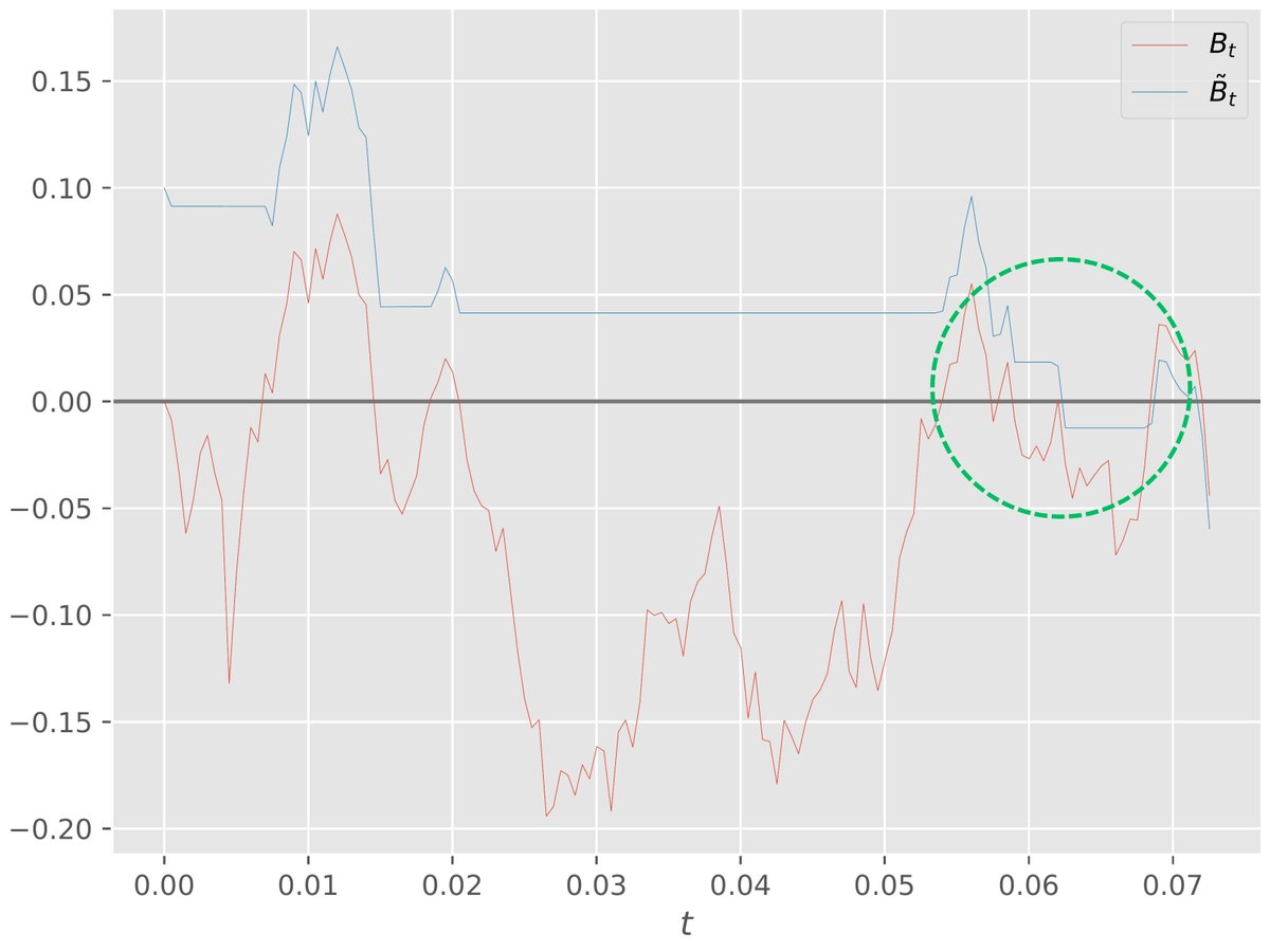
Let t be such that Wₜ > 0. Then, we must have that Lₜ > L₀=0 ⟹ Wₜ > Xₜ.
Suppose there exists some u. Since Wₜ > 0 occurs at arbitrarily small times, there will always exist some t < u where Wₜ > Xₜ, resulting in a contradiction.
Suppose now that Xₜ is started from ε:
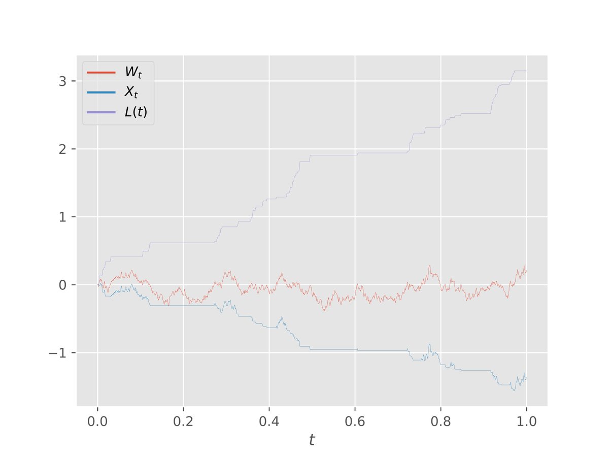
Xₜ ≔ ε + ∫₀ᵗ 1{Wₛ >= 0} dWₛ
Since Xₜ = ε + max(W_t,0) - ½ L(t) and L(t) strictly increases only when Wₜ=0, does there exist a time u such that
Xᵤ ≥ Wᵤ AND Xᵤ < 0?
https://t.co/1aPExUdxuR
More observations and questions on the following stochastic integral:
Xₜ ≔ ∫₀ᵗ 1{Wₛ >= 0} dWₛ
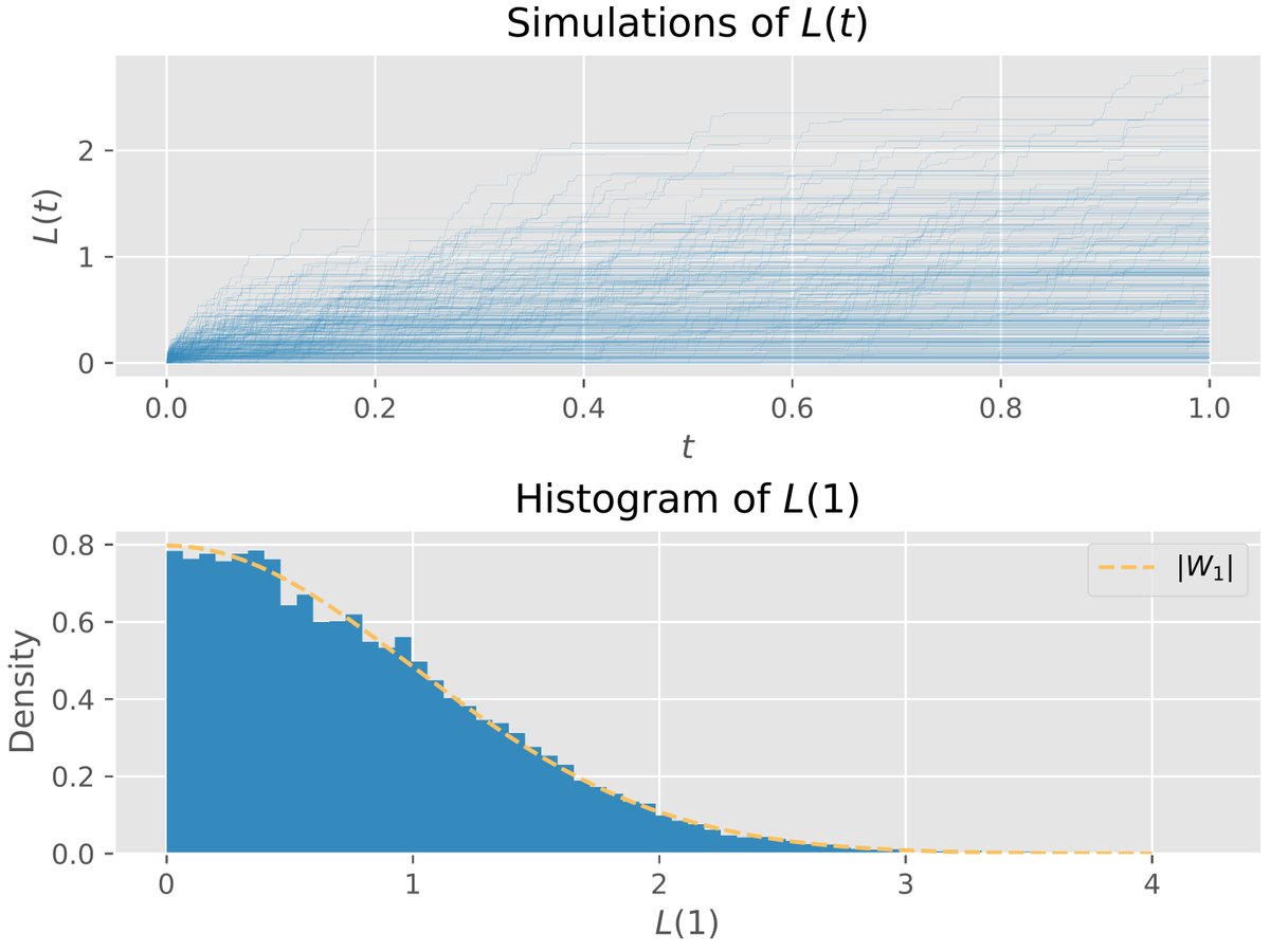
Numerically simulating this does confirm that E[Xₜ]=0 and Xₜ does go negative. What I did not expect, however, is the distribution of Xₜ to look the way it does.
@Almost_Sure I think I'm getting confused by the fact that Wₜ goes both negative (and positive) at arbitrarily small times, which (should?) mean that Xₜ also goes negative at arbitrarily small times (and hence inf { t | Xₜ < 0 } = 0 a.s. ?)
@Almost_Sure Ah. I realized I have another bad typo. The condition should be whether there exists a time u such that
Xₛ ≥ Wₛ ∀ s∈[0,u] AND Xᵤ < 0?
i.e., while X goes negative, does it stay at or above W the entire time?
#almostsure blog post: On the integral ∫I(W ≥ 0) dW
This looks at the mentioned integral, which displays properties particular to stochastic integration and which may seem counter-intuitive.
https://t.co/gRRyvtNg2O
More observations and questions on the following stochastic integral:
Xₜ ≔ ∫₀ᵗ 1{Wₛ >= 0} dWₛ
Numerically simulating this does confirm that E[Xₜ]=0 and Xₜ does go negative. What I did not expect, however, is the distribution of Xₜ to look the way it does.
Small question about Ito integrals: Consider
Xₜ ≔ ∫₀ᵗ 1{Wₛ >= 0} dWₛ
where Wₜ is a Brownian Motion and 1 is the indicator.
Xₜ is a martingale, so E[Xₜ] = 0. I would think that Xₜ is non-negative, but that doesn't seem to be true?
Using intuition from the discrete case, "Xᵤ downcrosses 0 when Wᵤ also downcrosses 0", and so u exists. However, I have no idea whether this holds in the continuous limit...
Numerical simulations show that u exists, but I feel like this is due to numerical error?


![oswinso's tweet photo. More observations and questions on the following stochastic integral:
Xₜ ≔ ∫₀ᵗ 1{Wₛ >= 0} dWₛ
Numerically simulating this does confirm that E[Xₜ]=0 and Xₜ does go negative. What I did not expect, however, is the distribution of Xₜ to look the way it does. https://t.co/vIVtMdGdxr](https://pbs.twimg.com/media/F-MpP_8bAAAWs-d.jpg)