Project Psyche 2025

Designer of Psyce LLM & R4 Fusion Reactor: BNNT monocoque, AI-driven control, TRL-9 bound. Engineer, puzzle-solver, fusion geek. #R4Reactor #FusionAI

[Project Psyche 2025 @Matthew15280451]

we were able to successfully bench mark the system against this exact solar event ,we freaking did it and we ended up with a new early warning system we still have some work to do on that yet and this is what we are working on.@NASASpaceAlerts

SolarWatch v1.0 Architecture

Modular ingestion layer (solarwatch_ingest.py) – normalizes data from AIA, HMI, GOES, etc.

Preprocessor – existing wavelength_preprocessor.py v1.1-G (multi-band EUV)

Fusion engine – new solarwatch_data_fusion.py v1.0-G (cross-instrument correlation)

Core analysis – signal_tools + harmonics_tools (unchanged)

Output – standardized JSON alert packet for public use or reactor integration

2. Doppler & Other Instrument Compatibility

HMI Doppler velocity – line-of-sight velocity maps (full-disk, 45 s cadence)

HMI magnetograms – line-of-sight magnetic field (full-disk, 45 s cadence)

GOES XRS – soft X-ray flux (1–8 Å and 0.5–4 Å channels)

SDO/AIA full suite – 171/193/211/304 Å (already supported)

I promised @Stanford that they would get first copy because they have been really nice and helped me get the AIA level 1 data that @grok and I used to benchmark the system.

The other big thing we are also working on is a heliographic position tracking / disturbance locator feature the tracking uses standard FITS WCS keywords already present in AIA Level-1 files CRVAL1/CRVAL2, CDELT1/CDELT2, CROTA2, etc.

Then it converts pixel coordinates of the peak precursor region to heliographic (Stonyhurst) lat/long
computes region evolution rate (Δlat, Δlon per frame)
cross-references with the multi-band preprocessor output and then produces a single contract-driven JSON envelope for public SolarWatch.

This runs in parallel with the existing wavelength preprocessor.

Satellite operators receive “Region 1423 at N12E45 is showing precursor_index = 0.92 expected flare within 3 hours” instead of generic alerts.

Power-grid and space-mission planners get actionable, location-specific warnings.

We will offer the second copy to NASA/NOAA as a public service as I promised someone that I would give it away .

https://t.co/0Tu8s4W8BK

[Wonder of Science @wonderofscience]

Loops of superheated plasma larger than the Earth dancing across the Sun, recorded by the Solar Dynamics Observatory spacecraft.

📽: SDO/NASA Goddard

[Project Psyche 2025 @Matthew15280451]

@XFreeze I am working here lol 🤣.....

[Project Psyche 2025 @Matthew15280451]

@XFreeze Worth every penny

[Project Psyche 2025 @Matthew15280451]

@mbabazi_odeth Amen !!

[KARMAUS Mind @KarmausMind]

@elonmusk Grok image

[Elon Musk @elonmusk]

Product Perfection Produces Prosperity

[❣︎ꨄ F ꨄ❣︎ @fairydust_0]

Every step forward is a quiet rebellion against yesterday’s fear.

[Project Psyche 2025 @Matthew15280451]

fact✨

[ooaes @21xooaes]

A NASA fellow claims the modern world runs on one equation. Your phone signal, wifi, satellites, this post reaching your screen. All of it obeys one line of math written in the 1860s, before the light bulb existed. His words.

The man is Ali Alqaraghuli, a former NASA postdoctoral fellow who now runs two hardware companies.

And the way he teaches it is what makes the video worth it.

He does not derive the equation. He teaches you to read it. His claim is that school taught you to read math wrong, and one symbol proves it: what you were told is a plus sign is actually something else. Once you see it, the whole equation turns from notation into a sentence.

Then he uses that sentence to walk you through how a signal actually gets from your phone to a satellite and back. One viewer called that section straight up magic. It is 4 minutes of it.

The comments are the proof. A physics student wrote it explained what a semester with his professor could not. An electrical engineer admitted this is where the equations finally clicked. One person wrote: I cried and I do not even know why.

His larger point: the wireless world is not magic and never was. It is one readable line, and reading it is a skill nobody bothered to teach you.

One equation. Everything wireless. 14 minutes. It is in the video.

[Project Psyche 2025 @Matthew15280451]

@BMattMcCall @elonmusk For some reason or another I would not put it past Elon to at least weigh the odds I mean it would prove a point, right ?

[X Freeze @XFreeze]

Starship is still floating in the Indian Ocean more than four days after its controlled splashdown

SpaceX is now sending a vessel out to recover it

[Project Psyche 2025 @Matthew15280451]

Your correct.

Beyond that domain kinetic effects, double layers, reconnection microphysics, non Maxwellian distributions, wave particle resonance is not “better MHD.” It is a different description.

Treating it as a small correction inside ideal MHD is the mistake .

That is exactly why the architecture we sketched stays honest in short 👇

Our Continuum MHD / stability kernel layer = Primary live path γ, N_p, α, topology

Kinetic =Own field: demand on actuators, precursor enrichment, offline / slow analysis

kinetic_demand_bridge its own module =Interface only does not pretend kinetic is continuum

You do not fold kinetic into MHD and call it done.

You keep the fluid model where it applies, and treat kinetic as a separate authority that writes requirements ,bandwidth, authority margin, early warning, without overriding the locked continuum contracts.

Your reply is the same split I already accepted and implemented.

Domain limited approximation, not a universal plasma theory.

In my studies no two plasmas are the same different density, temperature, profiles, impurity mix, wall conditioning, magnetic geometry, drive method, even the same device on different shots is different.

This is why I feel my control architecture is so important it adapts to that.

The continuum MHD is already an approximation kinetic effects sit on top of that variability.

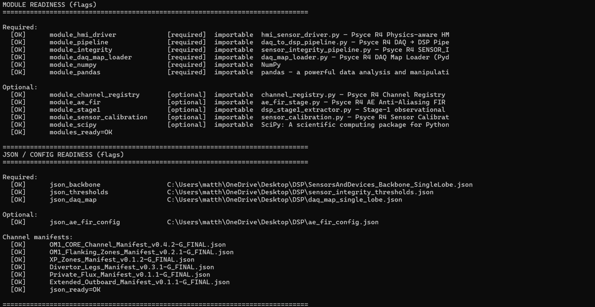
There is no universal plasma that the control law can assume and this I the exact reason why I refused to tune the machine to the HMI data we spoke about last week it was only meant to flex the sensors ,DSP pipeline nothing more two totally different regimes.

[Project Psyche 2025 @Matthew15280451]

@areoinfo @QuantumTumbler MHD is a fancy ass Navier Stokes with electromagnetism welded on.

[Project Psyche 2025 @Matthew15280451]

@ryanultralifeio @QuantumTumbler Please check your message Ryan I sent you a CSV with 40 frames

[devalopr @_devalopr]

ASML's EUV machines move at 20Gs of acceleration while maintaining positioning accuracy of 5 silicon atoms!

What actuators do they use to achieve this level of accuracy while moving this violently?

This Veritasium video did not answer that question but I found some answers👇

[Philosophy Of Physics @PhilosophyOfPhy]

Visualization of the incompressible Navier–Stokes equation.

Showing how pressure, inertia, viscosity, and external forces govern fluid motion, from smooth laminar flow to vortices, smoke advection, and turbulence.

[Project Psyche 2025 @Matthew15280451]

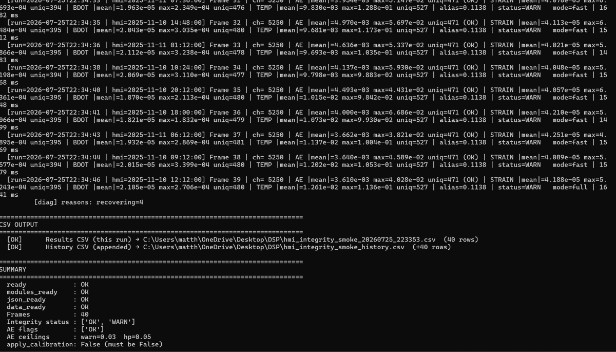
Frames are randomly selected from my directory of downloaded JSOC AIA files I have over 700MB of HMI 720`s and NPY files

The results have gotten much better then what we got the other day after chasing a few bugs 🤣

It would require me giving you full access to the full repo as listed and I'm a bit protective just ask @QuantumTumbler he know all about it 🤣

But I understand what your offering it very generous I'm open to discussion, DM me we can talk .

But I know the work has to be validated and I cant do that by my self.

[Project Psyche 2025 @Matthew15280451]

@QuantumTumbler Agreed that’s why we stopped at architecture talk and built the harness. Fault inject, golden vectors, property checks, stress under production schedule, recovery under residual.

Results are measured; slow-partition stuck latency under period=10 is one of the real findings.

[Project Psyche 2025 @Matthew15280451]

@QuantumTumbler

[Project Psyche 2025 @Matthew15280451]

@elonmusk What material did you use ?

[SpaceX @SpaceX]

Splashdown confirmed! Congratulations to the entire SpaceX team on the 13th flight test of Starship!