Sunwoo Hong ✈️EMNLP✈️

Building the next generation of AI @KAIST_AI, @VectorInst | @SeoulNatlUni ECE

[Sunwoo Hong ✈️EMNLP✈️ @SunwooHong_AI]

🌐 Project: https://t.co/XvrJPMo6Pe
📝 Paper: https://t.co/qJoIyjKh7f

🗓️ Sun Oct 25, 16:00–17:30
📍 F7 · Oral Session 4

Come say hi in Budapest!🇭🇺
@KAIST_AI @VectorInst

[Sunwoo Hong ✈️EMNLP✈️ @SunwooHong_AI]

🎉 Pivot-SD is an ORAL at #EMNLP2026!

We post-train a diffusion LM with a loss on just 10 tokens per response, and it beats both SFT and diffusion RL on math & code.

The trick isn't training on fewer tokens. It's training on the right ones.

[Sunwoo Hong ✈️EMNLP✈️ @SunwooHong_AI]

[5/6] And it's cheap: 200 questions × 4 rollouts, sampled once offline.

2.8 h total on 2 GPUs, ~8× less time than 5k-step diffu-GRPO, with a higher average accuracy (51.1 vs 47.4).

[Sunwoo Hong ✈️EMNLP✈️ @SunwooHong_AI]

[4/6] Is it the selection, or just sparsity? Same objective, different targets (MATH500, gain over base):
• Pivot-SD: +6.1
• All tokens in the state: +3.6
• Random token: +3.5
• Random step: −1.5, below the base model

[Sunwoo Hong ✈️EMNLP✈️ @SunwooHong_AI]

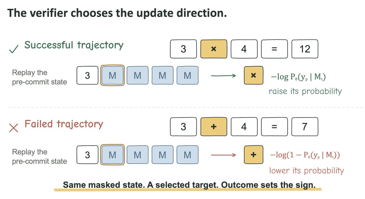
[3/6] Then we replay the exact masked state where each pivot was committed:

✅ correct answer → raise its probability (CE)
❌ wrong answer → lower it (unlikelihood)

Every other token gets no loss, so the valid steps of a failed answer stay untouched.

[Sunwoo Hong ✈️EMNLP✈️ @SunwooHong_AI]

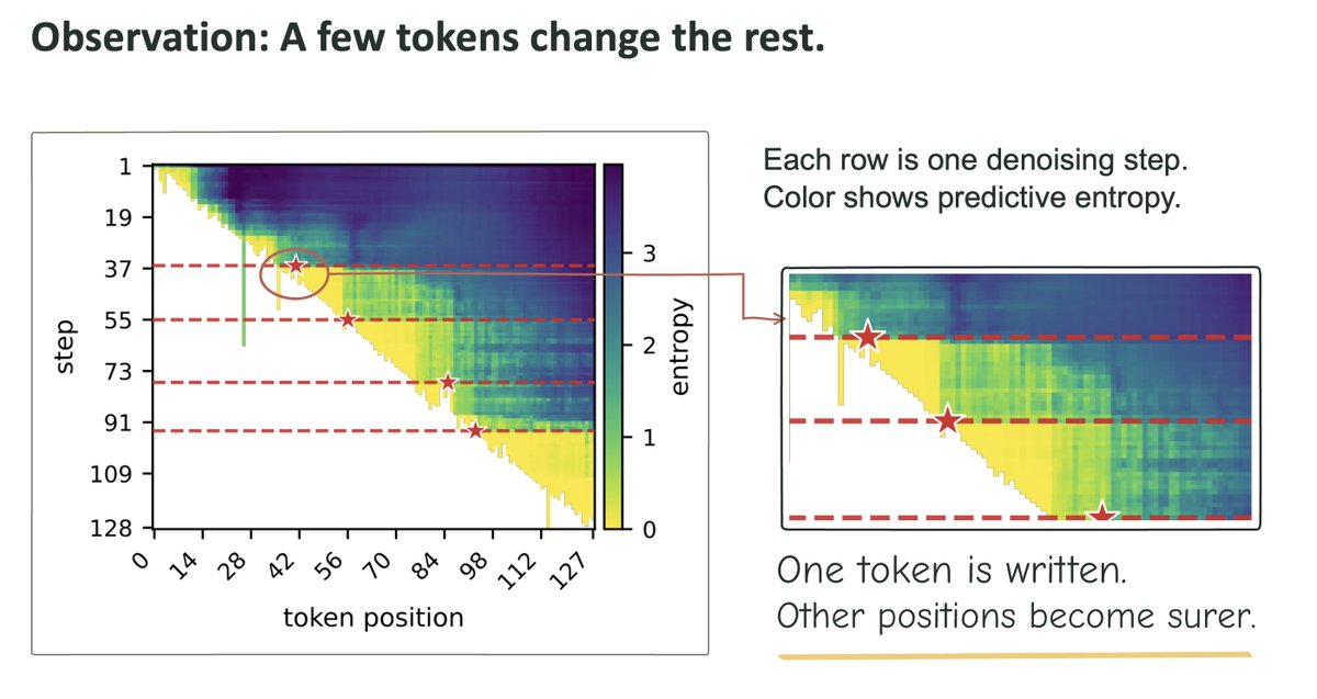
[2/6] In masked diffusion LMs, a few commitments during denoising suddenly make the remaining blanks much more certain.

We call them pivots. To find them, we score each step by information gain: how much the entropy over the still-masked positions drops.

[Sunwoo Hong ✈️EMNLP✈️ @SunwooHong_AI]

@vincesitzmann LLMs won because internet text is the output: trillions of tokens of exactly what the model must produce. Video is internet-scale too, but has no action labels. If paired action data is fundamentally capped far below that, isn’t that exactly where inductive bias earns its keep?

[Sunwoo Hong ✈️EMNLP✈️ @SunwooHong_AI]

https://t.co/bb68nmKh7F

[Sunwoo Hong ✈️EMNLP✈️ @SunwooHong_AI]

✨Accepted as a spotlight at #NeurIPS2025✨
We'll post the paper on Arxiv shortly.

[Jeffrey Emanuel @doodlestein]

Just read through the new LeJEPA paper by Yann LeCun and Randall Balestriero. I’ve been curious to know what Yann’s been working on lately, especially considering all his criticisms of LLMs (which I disagree with, as I think LLMs will keep improving and will take us to ASI fairly soon).

Anyway, there are several threads already on X about the paper and what it introduces. The short version is that it’s a principled, theoretically justified, and parsimonious approach to self-supervised learning that replaces a complex hodgepodge of ad-hoc, hacky heuristics for preventing mode collapse, which is the bane of self-supervised learning.

That’s where the model screws up and starts mapping all inputs to nearly identical embeddings or to a narrow subspace of embeddings, collapsing down all the richness of the problem into a pathologically simple and wrong correspondence.

The first pillar of the new approach is their proof that isotropic Gaussian distributions uniquely minimize worst-case downstream prediction risk.

As soon as I read that, I immediately thought of CMA-ES, the best available black-box optimization algorithm for when you don’t have access to the gradient of the function you’re trying to minimize, but can only do (expensive/slow) function evaluations.

Nikolaus Hansen has been working on CMA-ES since he introduced it way back in 1996. I’ve always been fascinated by this approach and used it with a lot of success to efficiently explore hyper-parameters of deep neural nets back in 2011 instead of doing inefficient grid searches.

Anyway, the reason why I bring it up is because there’s a striking parallel and deep connection between that approach and the core of LeJEPA.

CMA-ES says: Start with an isotropic Gaussian because it's the maximum entropy (least biased) distribution given only variance constraints. Then adapt the covariance to learn the problem's geometry.

LeJEPA says: Maintain an isotropic Gaussian because it's the maximum entropy (least biased) distribution for unknown future tasks.

Both recognize that isotropy is optimal under uncertainty for three reasons:

The maximum entropy principle; Among all distributions with fixed variance, the isotropic Gaussian has maximum entropy; I.e., it makes the fewest assumptions.

There’s no directional bias; Equal variance in all directions means you're not pre-committing to any particular problem structure.

You get worst-case optimality; Minimize maximum regret across all possible problem geometries.

So then what’s the difference? It comes down to adaptation timing. CMA-ES can adapt during optimization; it starts isotropic but then becomes anisotropic as it learns the specific optimization landscape.

In contrast, LeJEPA has to stay isotropic because it's preparing for unknown downstream tasks that haven't been seen yet.

This parallel suggests LeJEPA is applying a fundamental principle from optimization theory to representation learning. It's essentially saying:

“The optimal search distribution for black-box optimization is also the optimal embedding distribution for transfer learning.”

This makes sense because both problems involve navigating unknown landscapes; for CMA-ES, this is the unknown optimization landscape; for LeJEPA, this is the unknown space of downstream tasks.

This difference then makes me wonder: could we have "adaptive LeJEPA" that starts isotropic but adapts its embedding distribution once we know the downstream task, similar to how CMA-ES adapts during optimization? That would be like meta-learning the right anisotropy for specific task families.

Anyway, I thought I’d share my thoughts on this. It’s fascinating to see the connections between these different areas. The black-box optimization community has always been pretty separate and distinct from the deep learning community, and there’s not much cross-pollination there.

This makes sense, because if you have a gradient, you’d be crazy not to use it. But there are strong connections.

[Ernest Ryu @ErnestRyu]

I used ChatGPT to solve an open problem in convex optimization.

*Part I*

(1/N)

[Fei-Fei Li @drfeifei]

We are hiring researchers who are obsessed with generating pixels 🤩